Maps
When selecting the Maps Processing, a list of maps is shown as in Fig. 58.
To start building a map, one can select the “New Map” option (the green button on the top right corner). This will create RGB or Multispectral pages to upload the due camera images, as shown in Fig. 59 and Fig. 60.
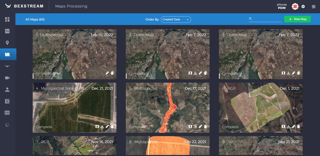
Fig. 58 List of maps page
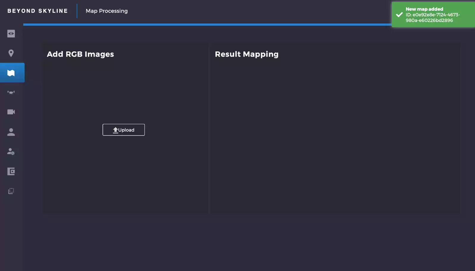
Fig. 59 RGB page created
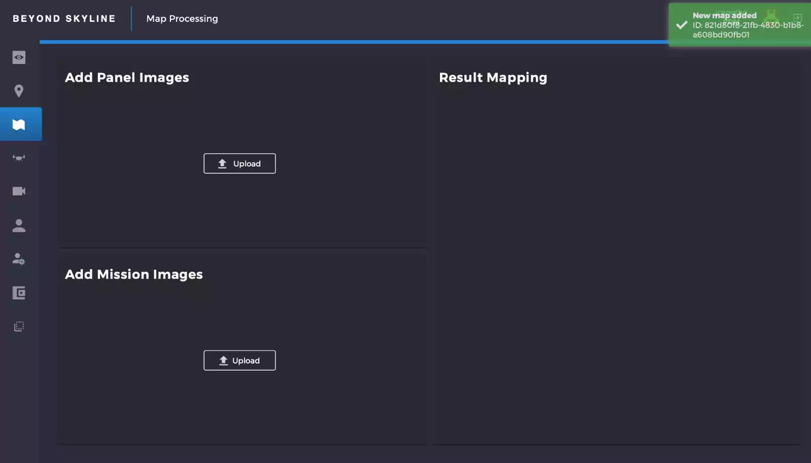
Fig. 60 Multispectral page created
In the next few steps, the option of creating an RGB map will be described: when RGB images are uploaded, 3 options available for the RGB page. These will appear on the right-hand side:
Select all to select all the next options (RGB and 3D options);
RGB to make the RGB map;
3D option to create a 3D map.
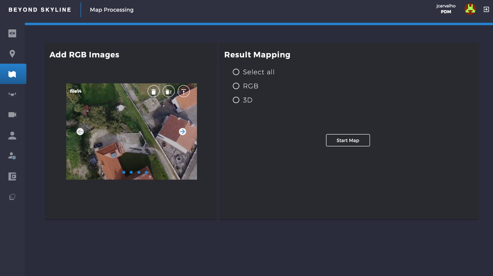
Fig. 61 RGB page – map type selection process
Pressing “Select all” option and clicking “Start Map” will start building the 2D and 3D RGB map. A progress bar informs the user about the status of the map creation. Fig. 62 shows the progress bar with a button to stop the current mapping process..
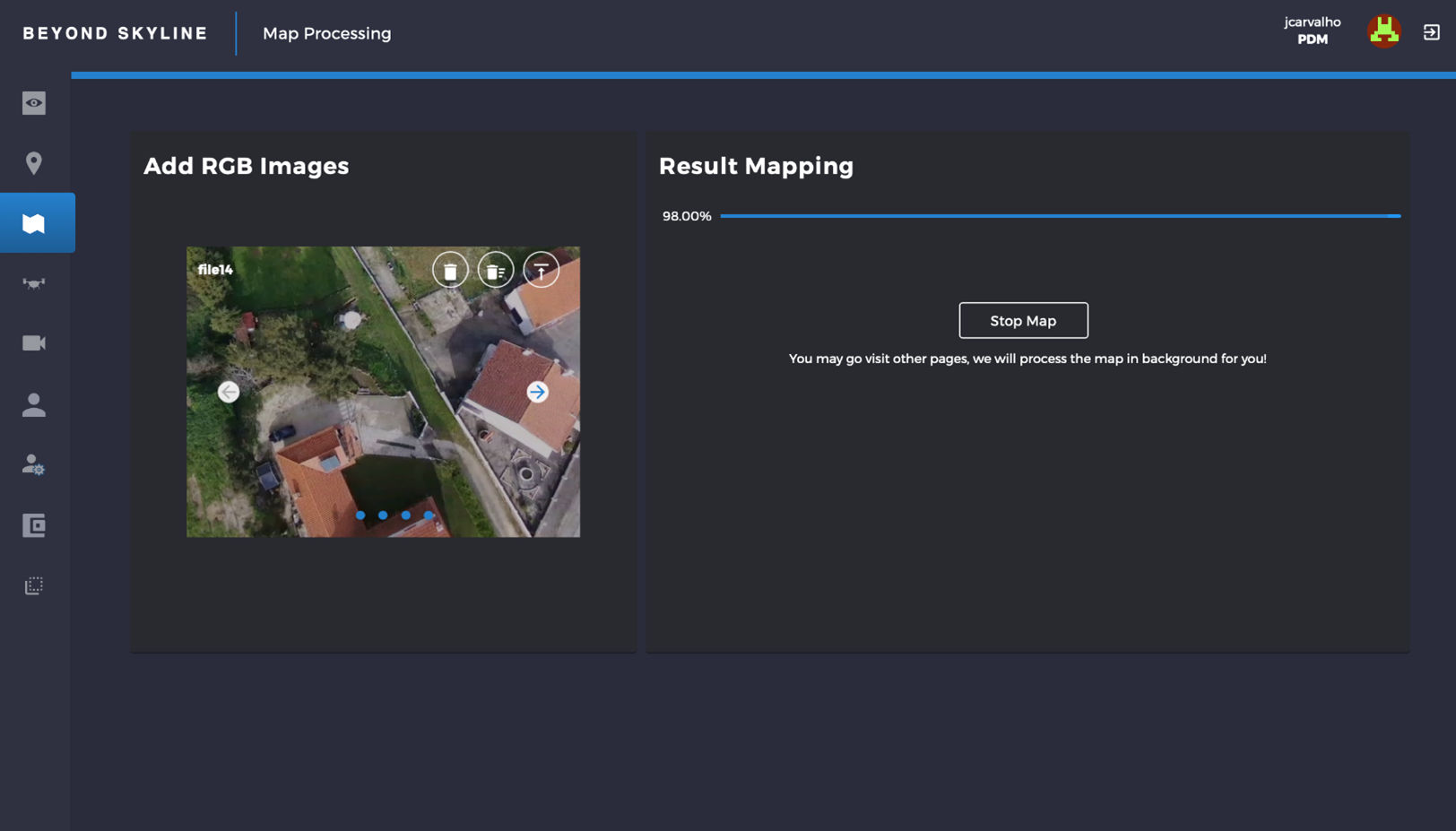
Fig. 62 Building an RGB map
When the progress bar reaches 100%, it will show the results. This can be seen in Fig. 63.
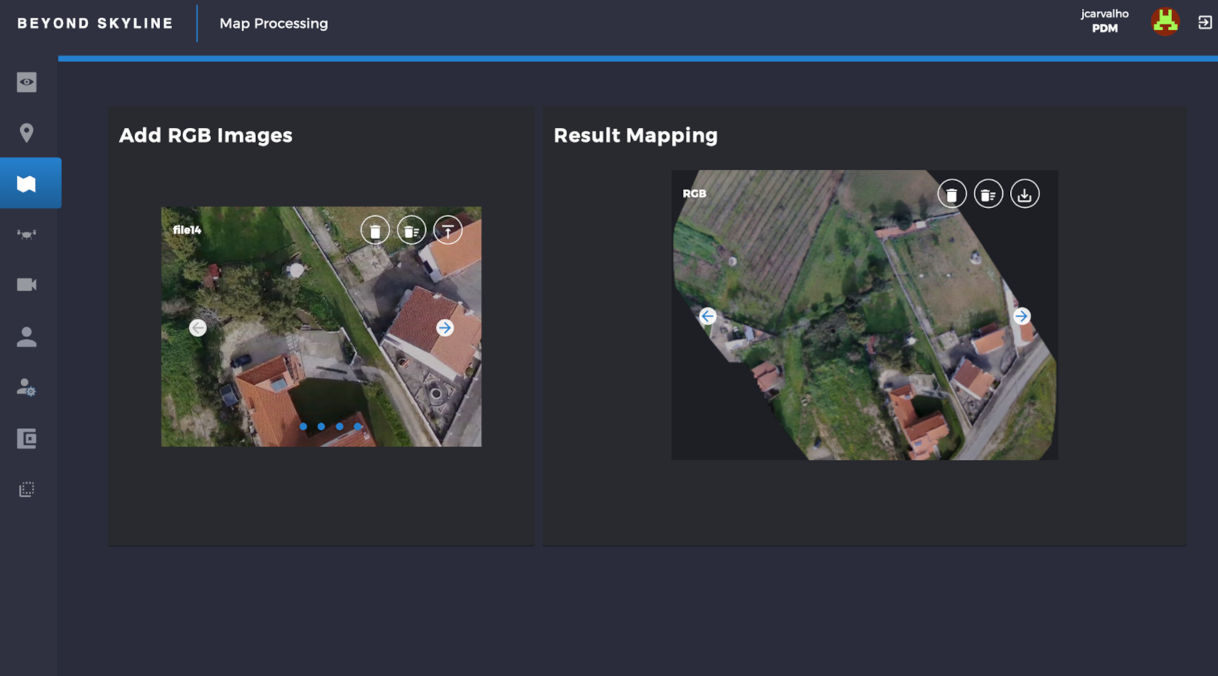
Fig. 63 End of building map
Back to the list of maps page, when maps are already created, four options are shown:
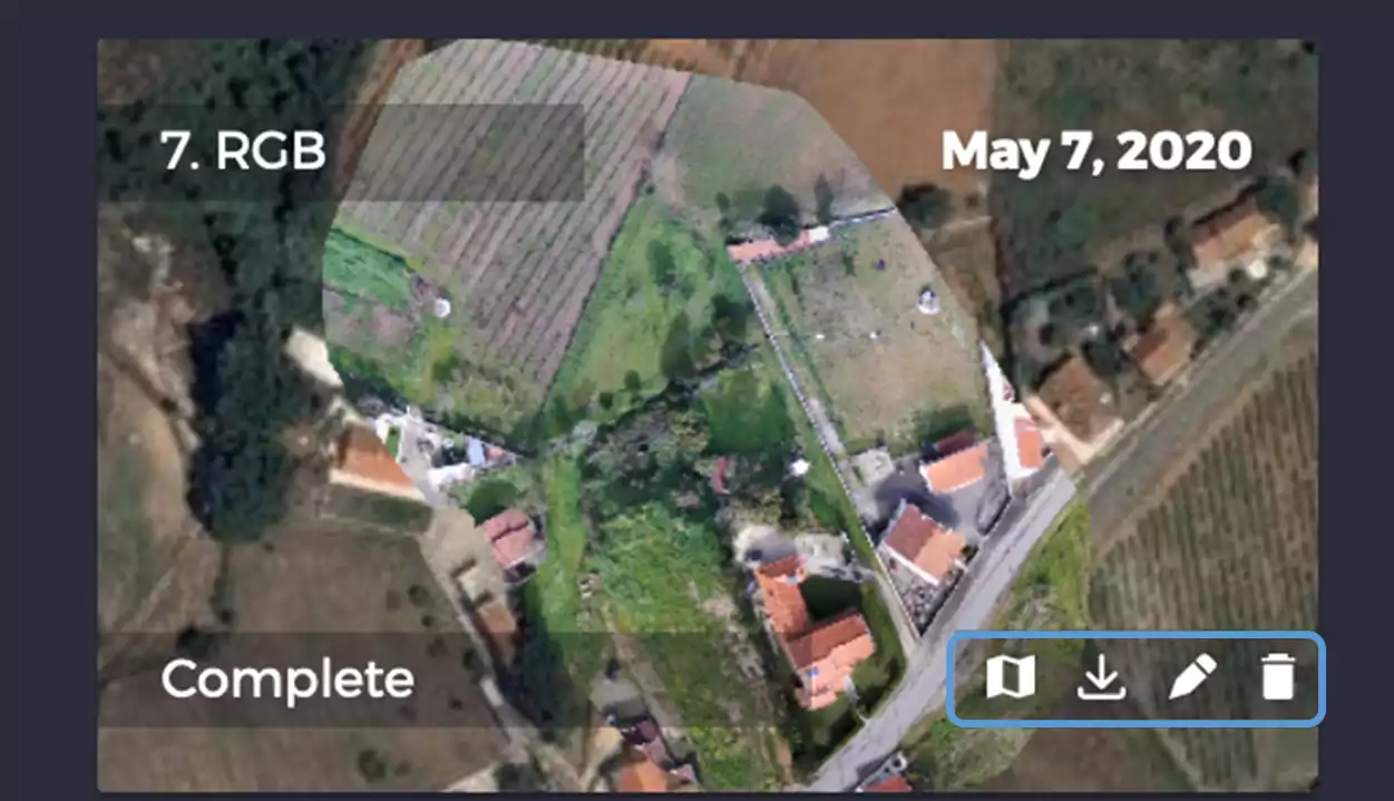
Fig. 64 Map list page with zoom on a specific map id
Visualize the 2D map;
Download the results map images;
Edit the RGB or Multispectral page;
Delete the map id.
When the first option is clicked, the 2D map indexes page is shown (Fig. 65). This page shows a timeline on the left-hand side with the list of all maps created nearby, chronologically ordered. It is possible to select more than one map to compare various indexes between different maps.
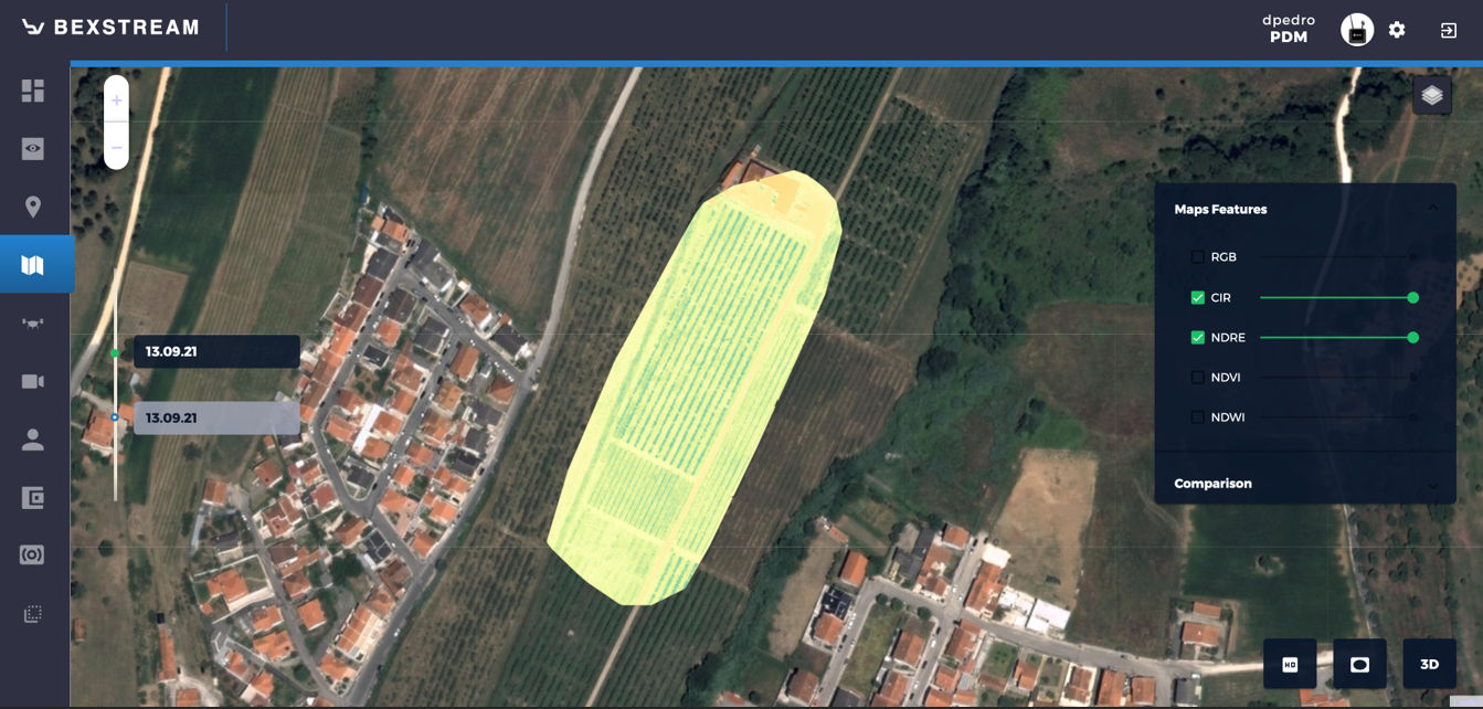
Fig. 65 2D map indexes page
The right-hand side displays a set of sliders, which allow the user to change the opacity of each index with the real-world map always in the background.
There are also two buttons available in the bottom right corner of the page. When the button on the left is toggled, it’s possible to measure areas as shown in Fig. 66, just by clicking on the points that create the limits of the selected area. By clicking this button again, one can draw a new area, without discarding the previous one.
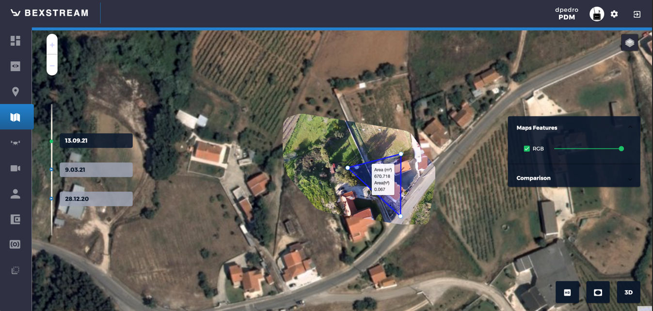
Fig. 66 2D area measurement
When selecting only one map on the left-hand side timeline, the user can enter the 3D view, by pressing the button on the right (bottom right side of the screen) and access the interface shown in Fig. 67.
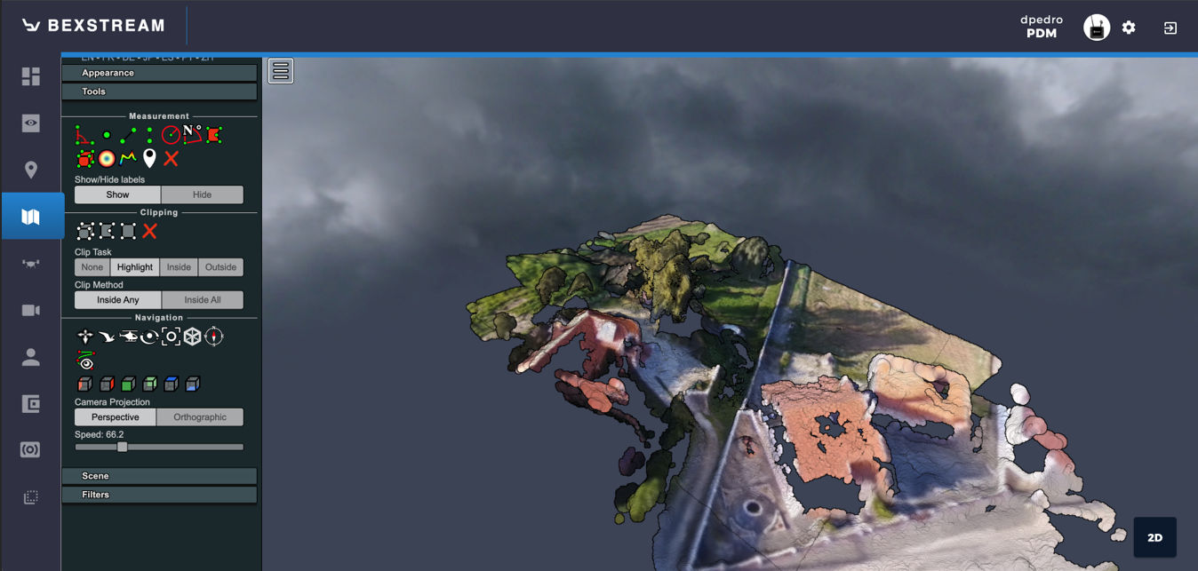
Fig. 67 3D map page
In this page the user is shown an approximate 3D view of the map. It is also possible to measure areas and volumes as shown in Fig. 68.
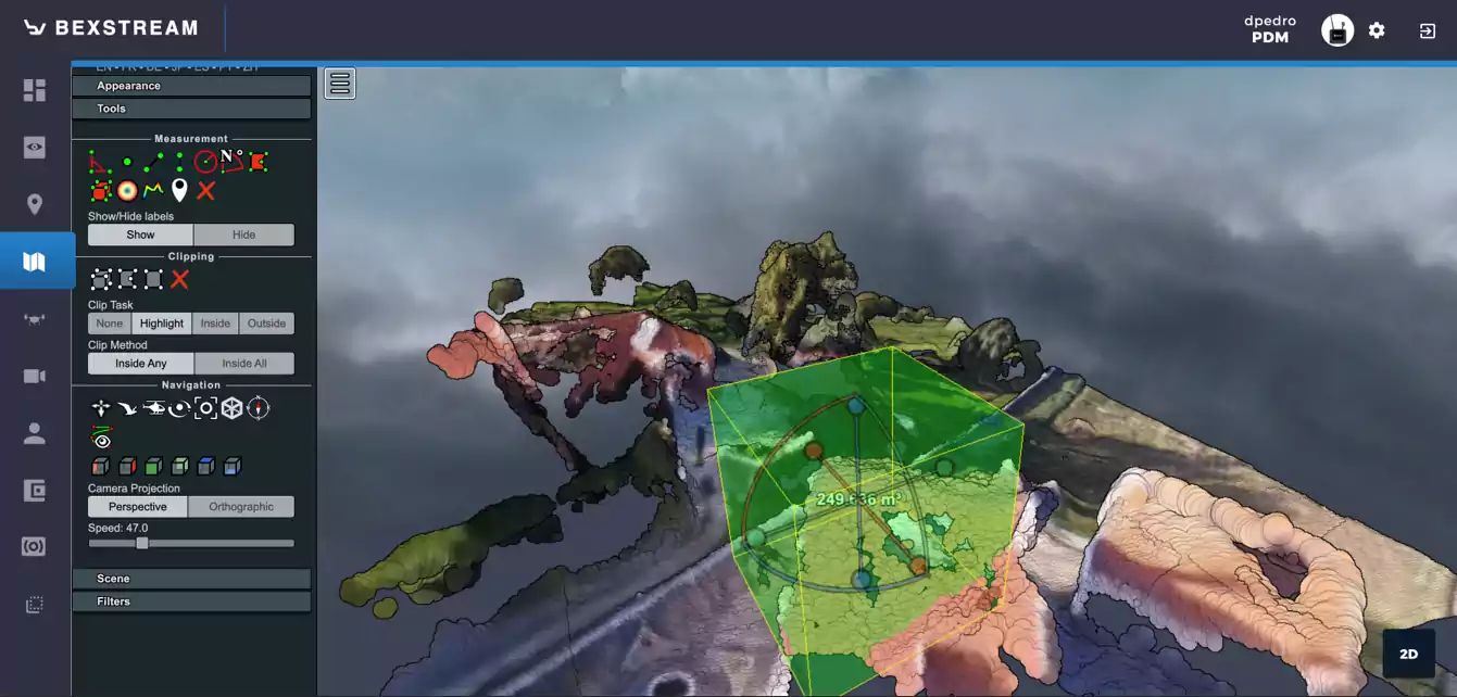
Fig. 68 Volume measurement
Working on 3D
Measurements
From 3D pointclouds is possible to extract some measurements of distances and volumes, among others. From the left sidebar, within the menu Tools, there are some icons for Measurement.
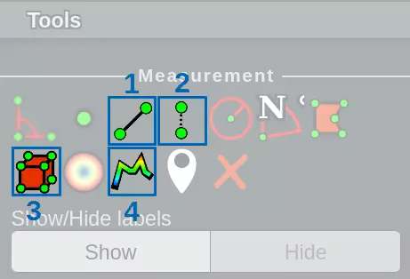
Fig. 69 Measurement Tools Menu
Fig. 69 highlights the Tools that will be further discussed.
1 Distance Measurement
This tool allows for distance measurement from one point to another. After selecting it, the points are picked using the letf-click. For quitting the point selection, use the mouse right-click.
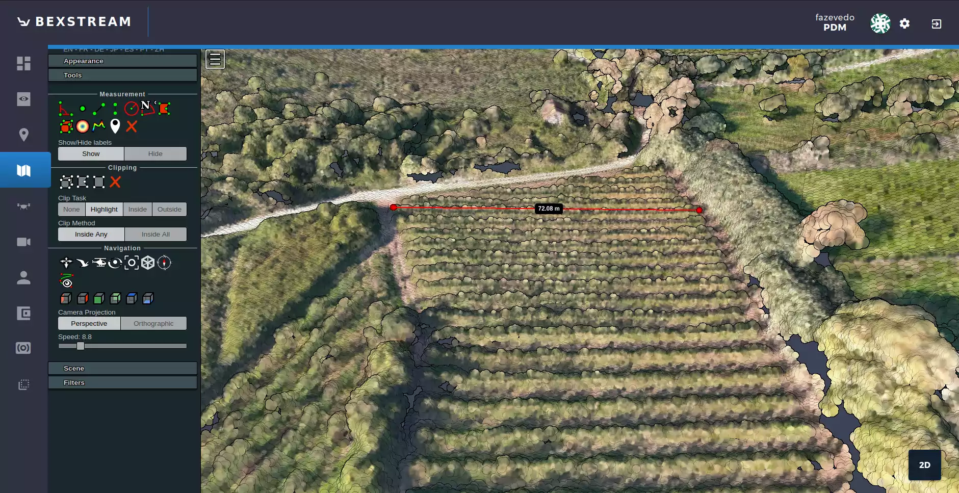
Fig. 70 Distance Measurement
After selecting one or more points, the distance between consecutive points will be shown on a label, as depicted in Fig. 70.
2 Height Measurement
This tool allows for measuring height differences of two points. In this mode, it displays the height difference after selecting 2 points, as shown in Fig. 71.
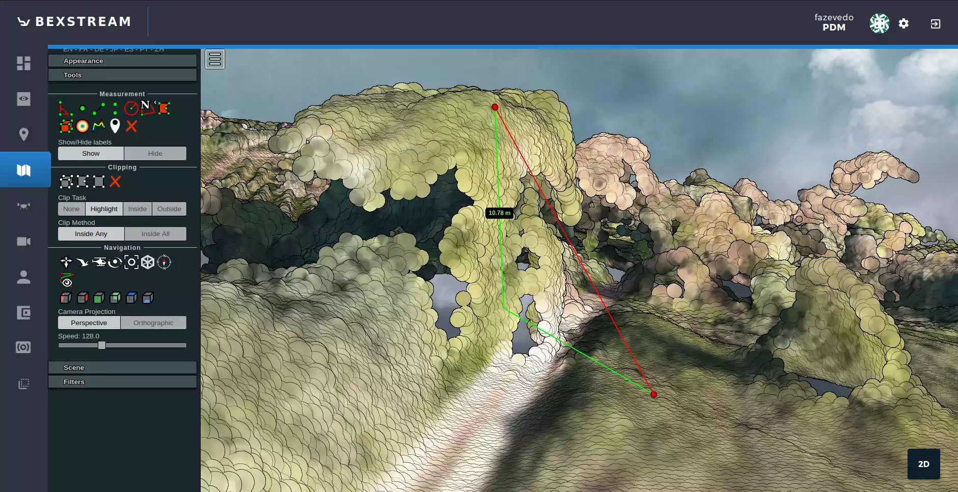
Fig. 71 Height Measurement
3 Volume Measurement
NOTE: This feature is under development and shall be used with caution.
The volume measurement is done by placing a box within the pointcloud area. After placing its center on a valid point, the rotation and dimensions of the box can be adjusted using the interface controls shown in Fig. 72.
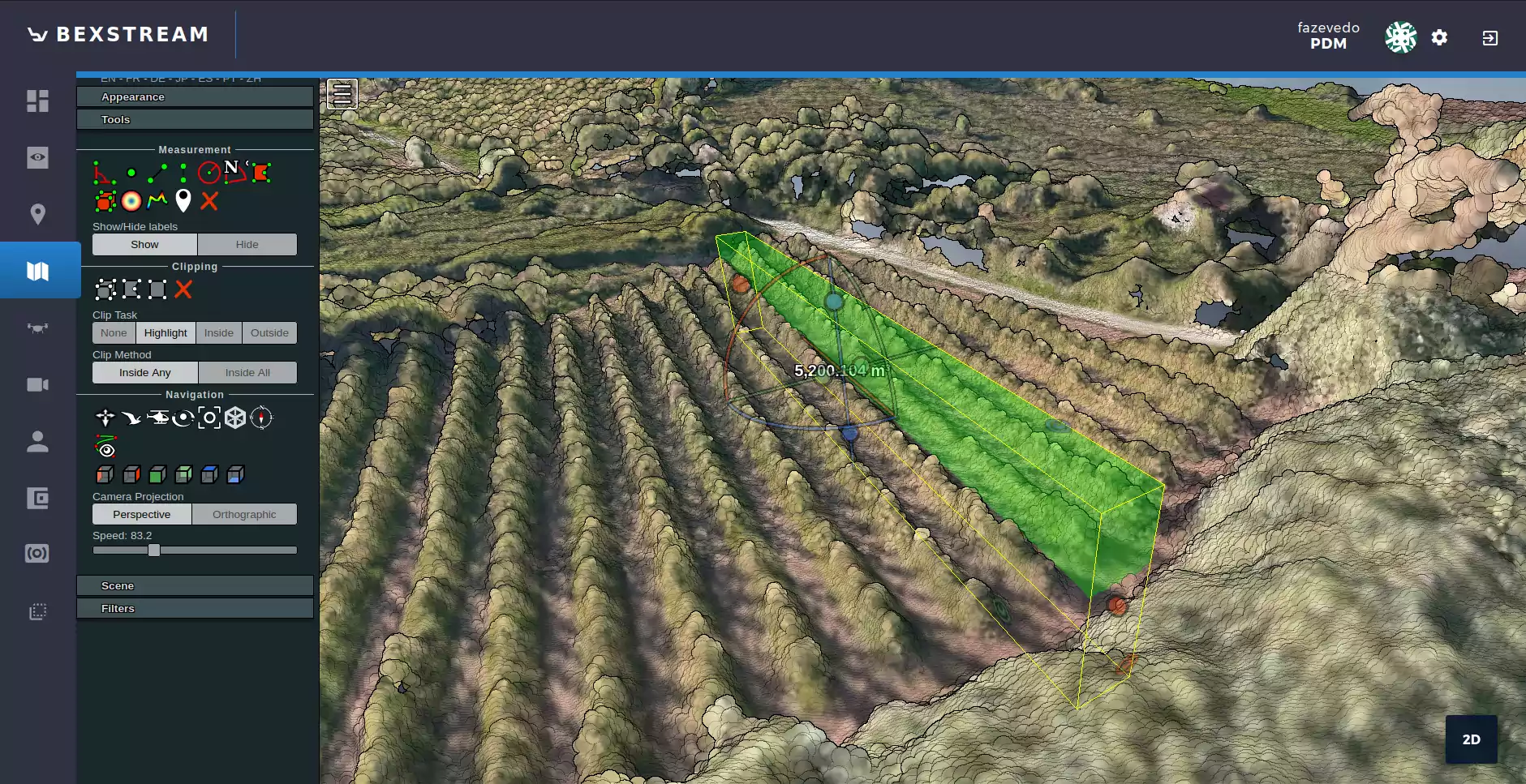
Fig. 72 Volume Measurement Controls
The total volume is shown on a label within the box (see Fig. 73).
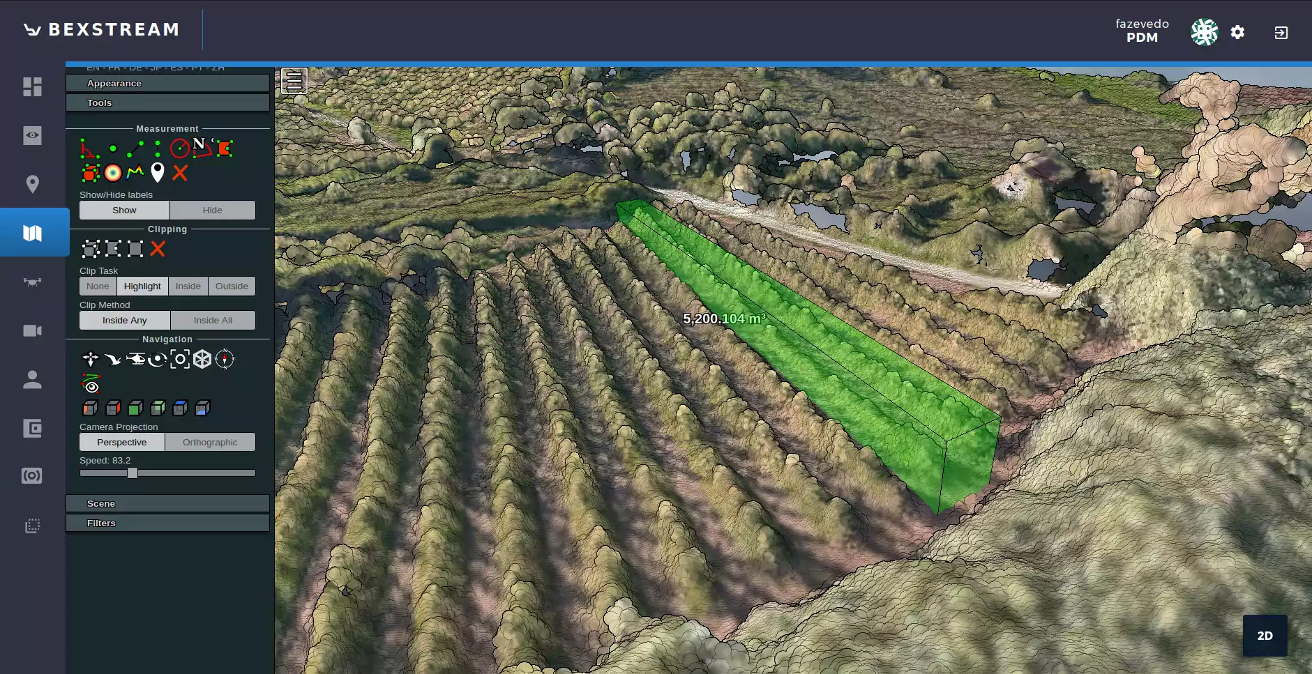
Fig. 73 Volume Measurement
In terms of visualization, the user can also highlight, or show only the content inside/outside the box.
For that the box has to be first converted into a Clip Volume (see Fig. 74).
This can be done under the Scene menu, selecting the Object Volume and then enable the make clip volume option.
Then, the desired visualization behavior of that volume (None, Highlight, Inside, Outside) is selected under the Tools/Clip Task menu.
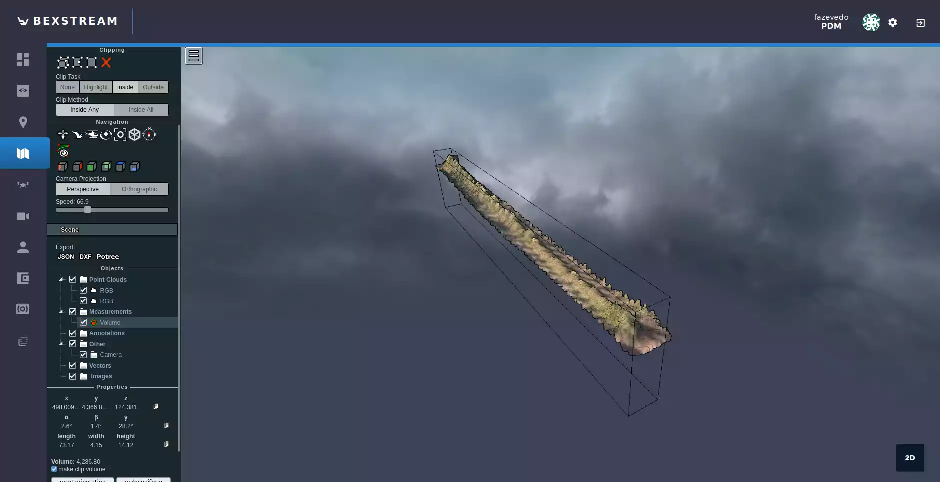
Fig. 74 Volume Measurement Clip Inside
4 Height Profile
It is also possible to analyze the height profile of a corridor.
After entering the profile selection, the user has to select two or more points in order to be possible the height analysis (see Fig. 75). The selection process is similar to the distance measurement’s.
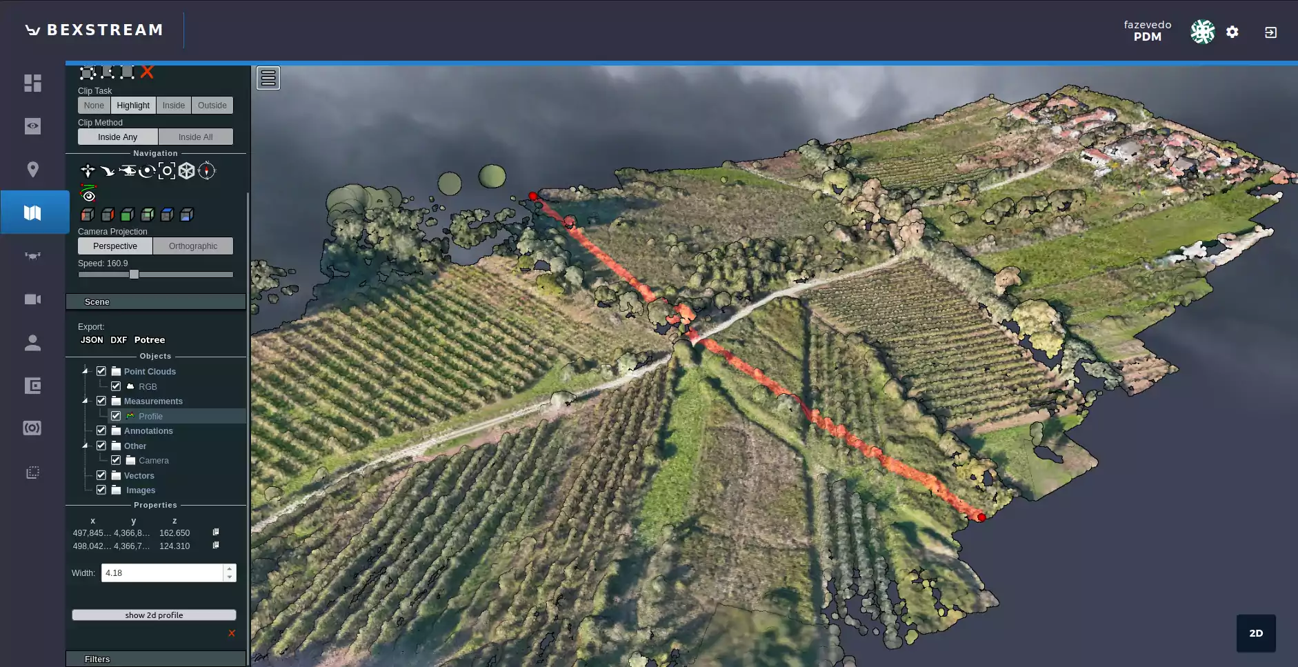
Fig. 75 Height Profile Selection
Under the Scene, some additional configuration can be done. Selecting the Profile, it is possible to configure its width (value in meters).
For a closer analysis, clicking on show 2d profile opens a new window containing a 2D perspective of the profile (Fig. 76), that can be downloaded either in LAS or CSV format (top-right corner).
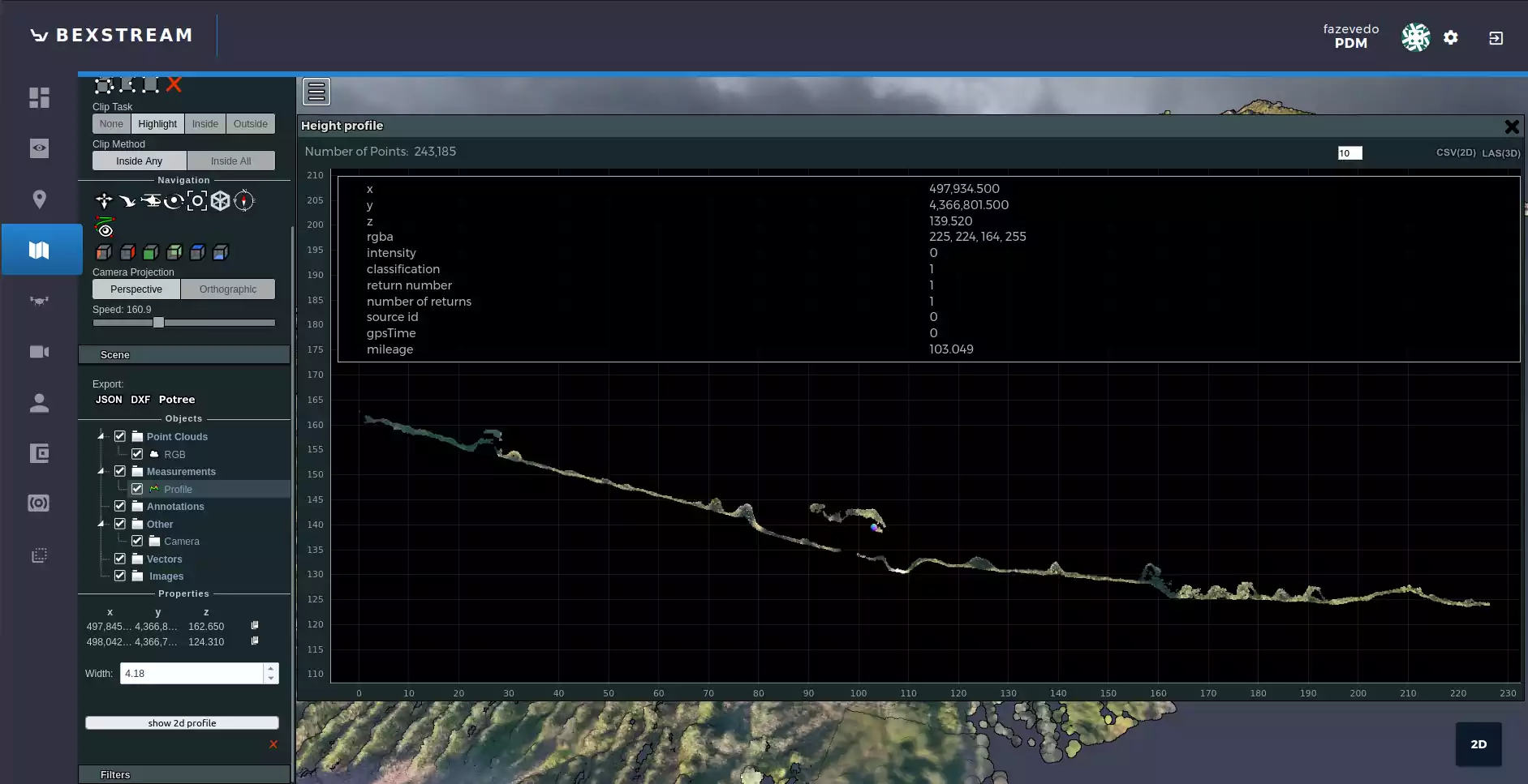
Fig. 76 Height Profile 2D Analysis
Coloring
The pointcloud coloring is made by the RGBA values of the correspondent camera pixels by default (Fig. 77).
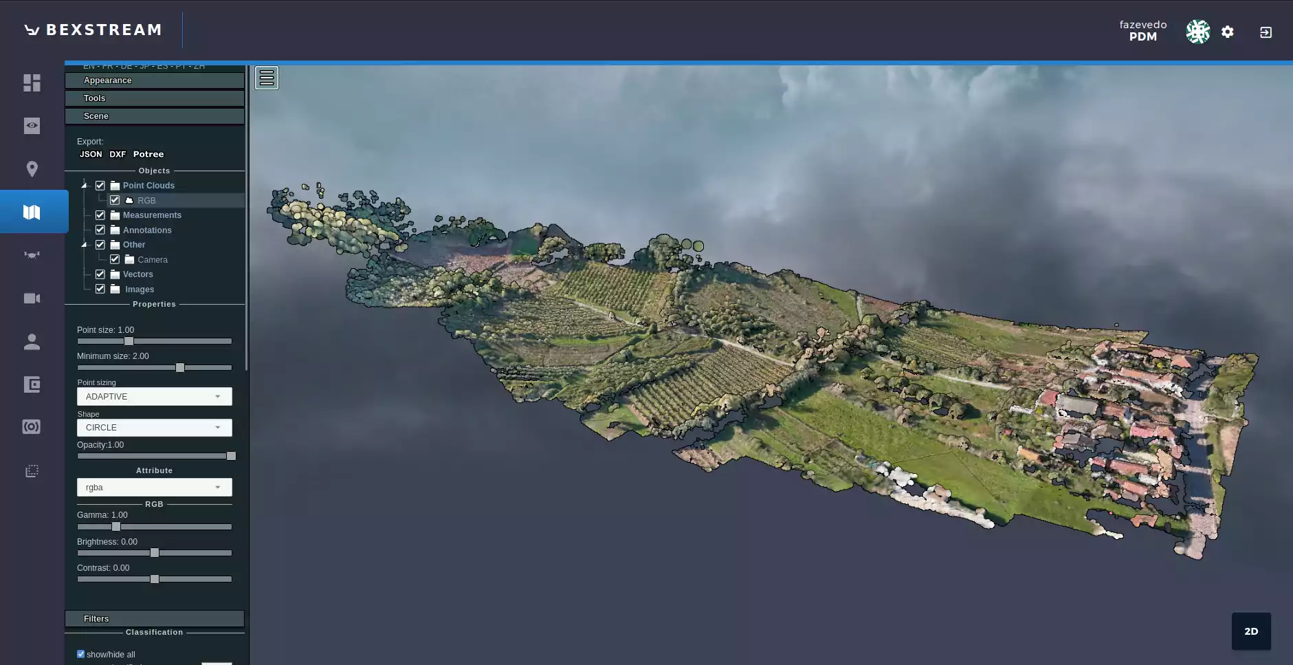
Fig. 77 Pointcloud Coloring RGBA
However, when this information is not present, the coloring is done taking into account the elevation of the points (Fig. 78).
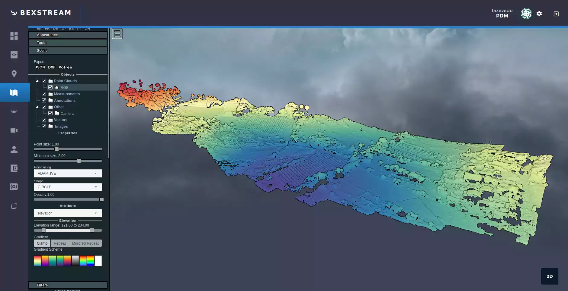
Fig. 78 Pointcloud Coloring Elevation
This change of coloring schemes can also be manually forced. Going into the Scene menu, select the desired pointcloud, and then select the Attribute for coloring.
Filters
There are some filters available to how only important part of the pointcloud. Those filters can be based on the classification of the points or on their source.
The point source corresponds to a small set of concatenated scans for a closer and independent analysis. This filter is controller through the first slider in the Filters/Point Source ID menu (Fig. 79).
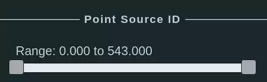
Fig. 79 Filtering by point source ID
Positioning
Georeferenced pointclouds display their location and relative positioning in the top-left corner, next to the sidebar (see positioning).
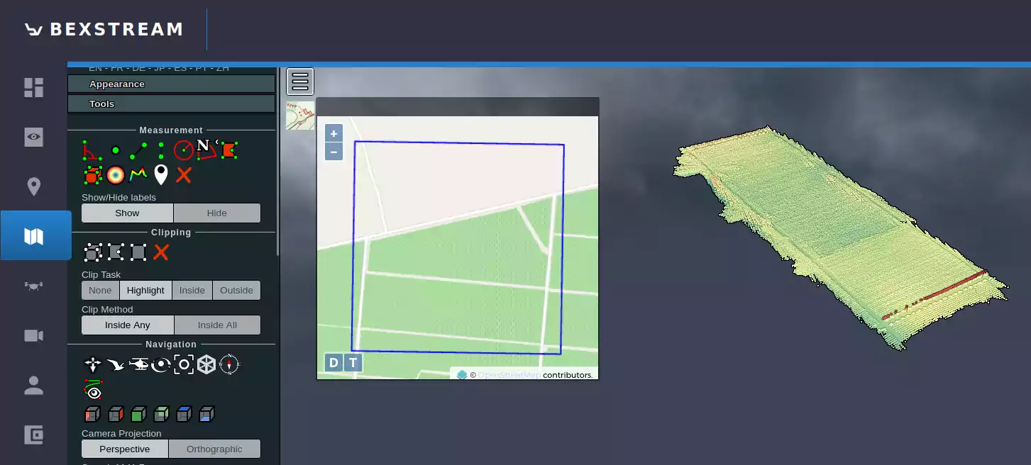
Fig. 80 Pointcloud geolocation