Machine Learning¶

`{article-info} :avatar: https://avatars.githubusercontent.com/u/3275593?s=80&v=4 :avatar-link: https://pradyunsg.me :avatar-outline: muted :author: Pradyun Gedam :date: Aug 15, 2021 :read-time: 5 min read `

This page contains a detailed analyses on SoA Machine Learning (ML) that are the pillars for the Beyond Vision developments. It will focus mainly on DL, but it’s important to understand the different fields inside AI and organize them in such a way that it’s possible to find parallelism between subsets and extract advantages from their differences [Dom12].

Artificial Intelligence (AI)

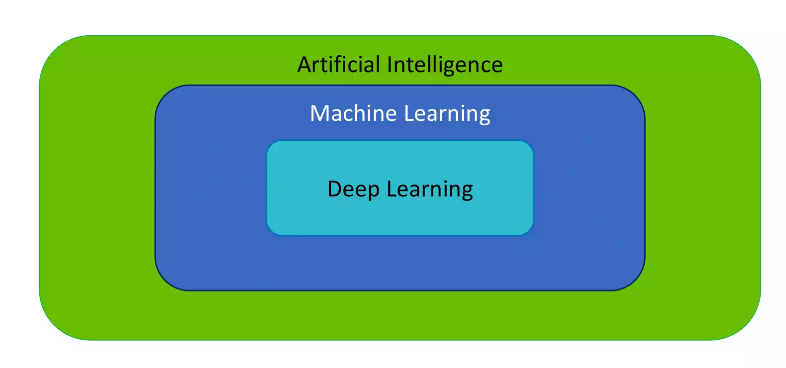
AI is a field of computer science that aims to make computers achieve human-style intelligence. As represented in figure, ML is a subset of AI, which contains a subset that try to replicate the human-brain called NN. NN contains large neural models which finally get us to the field of DL.

ML is a set of related techniques in which computers are trained to perform a particular task rather than by explicitly programming them. ML algorithms can be used to infer relationships and extract knowledge from gathered data.

A NN is a construction type in ML inspired by the network of neurons (nerve cells) in the biological brain. NN are a fundamental part of DL, and will be covered in this page.

Finally there is DL, which is a subfield of ML, that uses multi-layered neural networks. Often, ML and DL are used interchangeably.

Initially, we will go through the three main ways of learning, and then try to cluster the ML techniques into five clusters [Dom15]. There are main approaches for learning algorithms are SL, UL and RL [Ayo10].

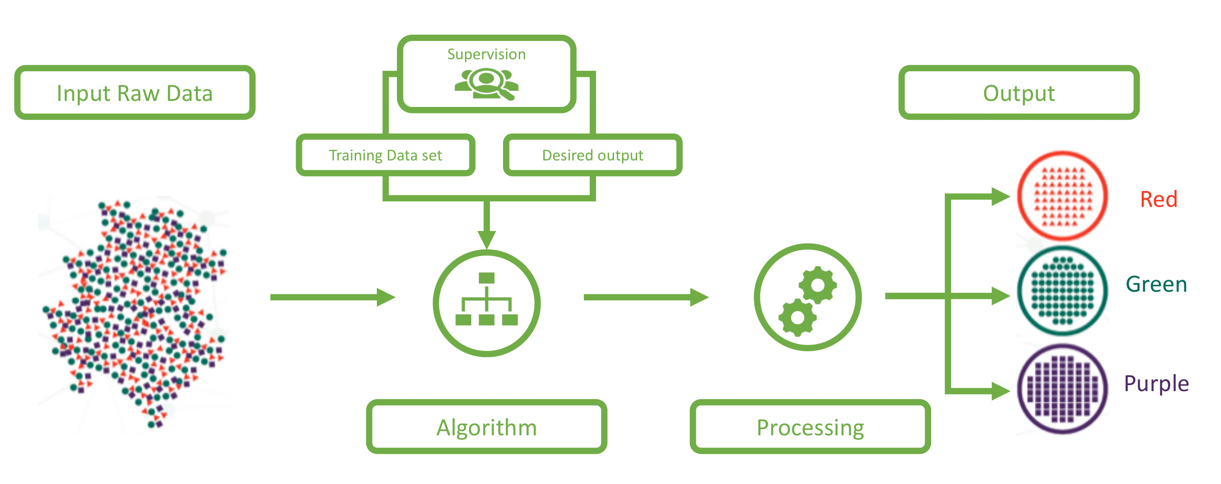
SL consist in obtaining outcome variables (or dependent variables) which are predicted from a given set of predictor variables (data features). Using these set of variables, a function that maps inputs to desired outputs is generated in what is called the training process. The process finishes when the model achieves a desired level of accuracy on the training data. Examples of SL algorithms are: KNN, Random Forest, Decision Tree and Logistic Regression. A sample representation of a SL workflow is illustrated on the figure.

On figure the dataset is divided by colors. After training the algorithm correctly classifies each object by it’s characteristic color.

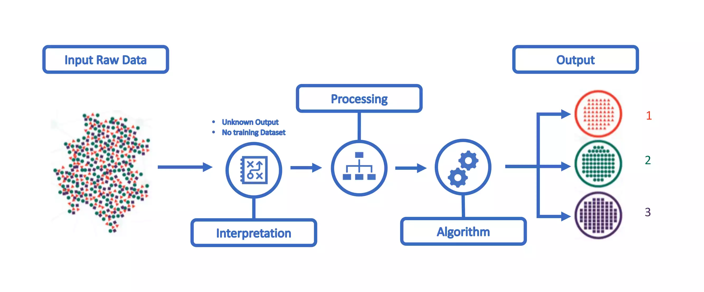
UL is a data-driven knowledge discovery approach that can automatically infer a function that describes the structure of the analyzed data or can highlight correlations in the data forming different clusters of related data. A UL workflow is depicted at the figure. Examples of algorithms include: K-Means, DBSCAN and Apriori.

On the figure no information is given to the algorithm, and it has to discover that the input contains objects of different shapes and colors. Afterwards, he will group the different objects according to it’s similarities. At the end, the output should be 3 clusters, with the different colors. Notice that in the case of SL the algorithm was able to recognize that a given object belong to the color class, whereas on the UL it just as the concept of the object belonging to a different category.

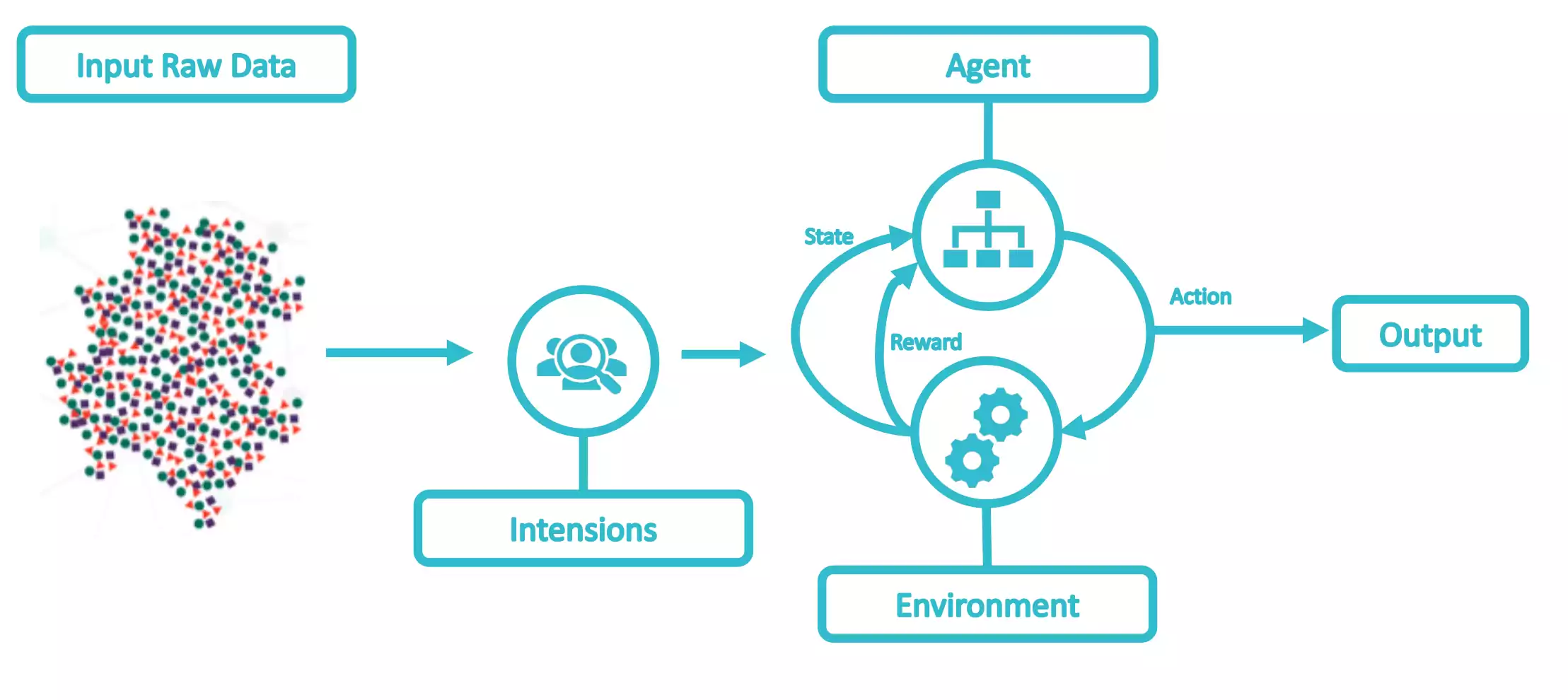
UnsupervisedLearning Unsupervised Learning.

Reinforcement Learning algorithms are trained to make specific decisions. The goal is to discover which actions lead to an optimal policy. This is done by learning from past experiences, as represented at the figure. As an example, a target policy is set, for instance the delay of a set of flows in an SDN. Then an algorithm results in actions on the SDN controller that change the configuration and for each action a reward is received, which increases as the in-place policy gets closer to the target policy. Ultimately, the algorithm will learn the set of configuration updates (actions) that result in such target policy (e.g. Markov Decision Process).

Compared to SL and UL, RL is slightly different, in the sense he does not intend to map the input to the output. For example, he can try to take actions towards the region area that contains the maximum number of red objects, but he does it undefinability, until he reaches an end function.

Reinforcement Learning Reinforcement Learning.

As described in [Dom12], there are 12 important key points that should be kept in mind when working with ML:

Learning = Representation + Evaluation + Optimization.
1. Representation - A classifier must be represented in a formal language that the computer can handle. Creating a set of classifiers the learner can learn is crucial.
2. Evaluation - An Evaluation function is needed to distinguish good classifiers from bad ones.
3. Optimization - A method to search among the classifiers in the language for the highest scoring one. The choice of optimization technique is key to the efficiency of the algorithm.
It is generalization that matters.
Data alone is not enough.
Overfitting has many faces.
Intuition fails in high dimensions.
Theoretical guarantees are not what they seem.
Feature engineering is the key.
More data beats a cleverer algorithm.
Learn many models not just one.
Simplicity does not imply accuracy.
Representable does not imply learnable.
Correlation does not imply Causation .

Machine Learning Fields¶

ML has many subfields, branches, and special techniques. To over simplify — in SL you know what you want to teach the computer, while UL is about letting the computer figure out what can be learned. SL is the most common type of ML the most used at Beyond Vision.

The majority of ML algorithms can be clustered into five clusters [Dom15], as summarized on table 1.1 :

Table 1 Different types of Machine Learning.¶
Cluster	Origins	Strength	Main Algorithm
Symbolist	Logic & philosophy	Structure Inference	Inverse deduction
Connectionists	Neuroscience	Estimating Parameters	Neural Networks
Evolutionaries	Evolutionary biology	Weighing Evidence	Genetic programming
Bayesians	Statistics	Structure Learning	Probabilistic Inference
Analogizers	Psychology	Mapping to Novelty	Kernel Machines

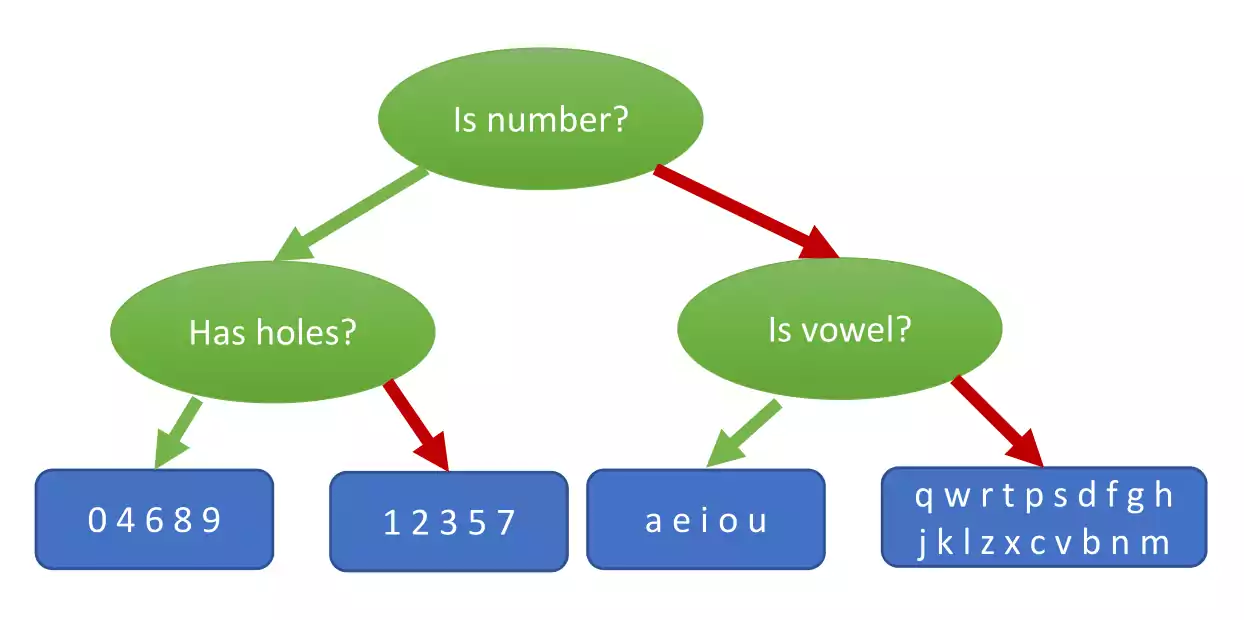
The symbolist cluster represent algorithms who believe in discovering new knowledge by filling in the gaps in the knowledge that you already have. They are the ones that most relate to computer science in the five clusters. Their master algorithm is inverse deduction. For the symbolist, learning is the inverse of deduction, which means that learning is the induction of knowledge. In practical terms, they try to create general rules from specific facts. On figure 1.5, is a simplistic representation of a typical symbolist algorithm, a decision tree. On this example, a character classifier is presented, where the output are 4 different possible groups. A decision tree has multiple types of nodes [KaminskiJS18]. On figure 1.5, decision nodes are represented in green and end nodes are represented in blue. The green arrows represent a true evaluation at the node, while the red arrows represent a false evaluation. A decision tree is a flowchart-like structure in which each internal node represents a “test” on an attribute (e.g. whether a coin flip comes up heads or tails), each branch represents the outcome of the test, and each leaf node represents a class label (decision taken after computing all attributes). The paths from root to leaf represent classification rules.

Symbolist Representation

In decision analysis, a decision tree and the closely related influence diagram are used as a visual and analytical decision support tool, where the expected values (or expected utility) of competing alternatives are calculated.

Among decision support tools, decision trees (and influence diagrams) have several advantages, such as:

Are simple to understand and interpret. People are able to understand decision tree models after a brief explanation.
Have value even with small datasets. Important insights can be generated based on experts describing a situation (its alternatives, probabilities, or costs) and their preferences for outcomes.
Help determine worst, best and expected values for different scenarios.
Use a white box model. If a given result is provided by a model.
Can be combined with other decision techniques.

On the other hand, decision trees have some disadvantages:

They are unstable, meaning that a small change in the data can lead to a large change in the structure of the optimal decision tree.
They are often relatively inaccurate. Many other predictors perform better with similar data. This can be remedied by replacing a single decision tree with a random forest of decision trees, but a random forest is not as easy to interpret as a single decision tree.
For data that include categorical variables with different number of levels, information gain in decision trees is biased in favor of those attributes with more levels [DRT11].
Calculations can get very complex, particularly if many values are uncertain and/or if many outcomes are linked.

The evolutionaries, have origins in the evolutionary biology. The main algorithm of this school, is the genetic programming and consist on replicating the process of genetic evolution.

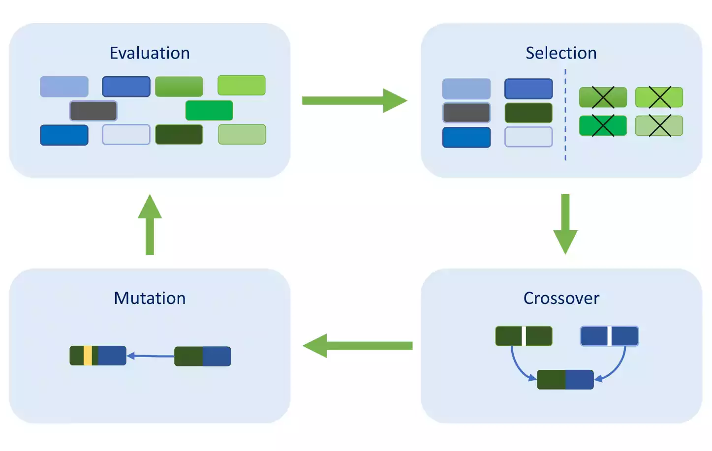
As it is illustrated in figure 1.6, it starts from a population of unfit (usually random) elements, and they are iteratively fit for a particular task by applying operations analogous to natural genetic processes to the population. It is essentially a heuristic search technique that searches for an optimal or at least suitable element.

The typical operations of a Genetic algorithm are:

Selection: the fittest elements for reproduction (crossover) and mutation are selected according to a predefined fitness measure, usually proficiency at the desired task.
Crossover: involves swapping random parts of selected pairs (parents) to produce new and different offspring that become part of the new generation of elements.
Mutation: consists involves substitution of some random part of a element with some other random part of another element.

Genetic Algorithm Representation.

Some combinations, usually the best ones, are directly copied from the current generation to the new generation, which is usually called elitism. Then the selection and other operations are recursively applied to the new generation of elements.

Typically, members of each new generation are on average more fit than the members of the previous generation, and the best-of-generation element is often better than the best-of-generation elements from previous generations. Termination of the recursion is when some individual element reaches a predefined proficiency or fitness level. A branch of Genetic algorithms are considered to be evolutionary bio-inspired, such as GBCA, FSA, CSO, WOA, AAA, ESA, CSOA, MFO and GWO [Dar18].

It can be considered that the main advantages of genetic algorithms are:

It can find fit solutions in less time. (fit solutions are solutions which are good according to the defined heuristic).
The random mutation guarantees to some extent that a wide range of solutions is generated.
Coding them is really easy compared to other algorithms.

On the other hand, the drawbacks of genetic algorithms are:

It is really hard for people to come up with a good heuristic which actually reflects what the algorithm should do.
It might not find the most optimal solution to the defined problem in all cases.
Its also hard to choose parameters like number of generations, population size or stopping condition. When the model is being worked, even though the heuristic was right, it might be hard to realize it because it’s running for a few generations.

The bayesians come from statistics and most of their algorithms are extensions and reformulations of the equation [eq:bayes]. In probability theory and statistics, Bayes’ theorem describes the probability of an event, based on a priori knowledge that may be related to the event. The theorem shows how to change a priori probabilities in view of new evidence to obtain a posteriori probabilities.

The core stone is the equation [eq:bayes] [KSO94], on which \(A\) and \(B\) are events, \(P(A|B)\) is a conditional probability of the likelihood of event \(A\) occurring given that \(B\) is true, \(P(B|A)\) is the conditional probability of the likelihood of event \(B\) occurring given that \(A\) is true and finally \(P(A)\) and \(P(B)\) are the probabilities of observing \(A\) and \(B\) independently of each other. This is known as the marginal probability.

\[\begin{split}\label{eq:bayes} \left\{\begin{matrix} P(A|B) = P(A) \frac{P(B |A)}{P(B)} \space\\ P(B) \neq 0 \end{matrix}\right. \space,\end{split}\]

Some advantages to using Bayesian analysis include the following:

It provides a natural and principled way of combining prior information with data, within a solid decision theoretical framework. You can incorporate past information about a parameter and form a prior distribution for future analysis. When new observations become available, the previous posterior distribution can be used as a prior. All inferences logically follow from Bayes’ theorem.
It provides inferences that are conditional on the data and are exact, without reliance on asymptotic approximation. Small sample inference proceeds in the same manner as of a larger dataset. Bayesian analysis also can estimate any functions of parameters directly, without using the “plug-in” method (a way to estimate functionals by plugging the estimated parameters in the functionals).
It obeys the likelihood principle. If two distinct sampling designs yield proportional likelihood functions for, then all inferences about should be identical from these two designs. Classical inference does not in general obey the likelihood principle.
It provides a convenient setting for a wide range of models, such as hierarchical models and missing data problems. MCMC, along with other numerical methods, makes computations tractable for virtually all parametric models.

There are also disadvantages to using Bayesian analysis:

It does not tell you how to select a prior. There is no correct way to choose a prior. Bayesian inferences require skills to translate subjective prior beliefs into a mathematically formulated prior. If you do not proceed with caution, you can generate misleading results.
It can produce posterior distributions that are heavily influenced by the priors. From a practical point of view, it might sometimes be difficult to convince subject matter experts who do not agree with the validity of the chosen prior.
It often comes with a high computational cost, especially in models with a large number of parameters. In addition, simulations provide slightly different answers unless the same random seed is used. Note that slight variations in simulation results do not contradict the early claim that Bayesian inferences are exact. The posterior distribution of a parameter is exact, given the likelihood function and the priors, while simulation-based estimates of posterior quantities can vary due to the random number generator used in the procedures.

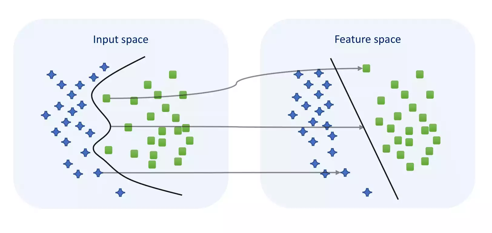
The analogizers actually have influences from a lot of different fields, being psychology probably the most important to them. The core algorithm for the analogizers is the kernel machines as known as SVM [CV95], as is exemplified at figure 1.7.

Support Vector Machine Representation.

Given a set of training examples, each marked as belonging to one or the other of two categories, an SVM training algorithm builds a model that assigns new examples to one category or the other, making it a non-probabilistic binary linear classifier (although methods such as Platt scaling exist to use SVM in a probabilistic classification setting). An SVM model is a representation of the examples as points in space, mapped so that the examples of the separate categories are divided by a clear gap that is as wide as possible. New examples are then mapped into that same space and predicted to belong to a category based on the side of the gap on which they fall.

In addition to performing linear classification, SVMs can efficiently perform a non-linear classification using what is called the kernel trick, implicitly mapping their inputs into high-dimensional feature spaces.

When data is unlabeled, SL is not possible, and an UL approach is required, which attempts to find natural clustering of the data to groups, and then map new data to these formed groups [SAHG11].

In general terms, the main advantages of SVMs can be described as:

SVMs are very good when there’s not much information about the working data.
Works well with even unstructured and semi structured data like text, images and trees.
The kernel trick is the major advantage of SVM. With an appropriate kernel function, it’s possible to solve any complex problem, with few parameters.
Unlike in neural networks, SVM is not solved for local optima.
It scales relatively well to high dimensional data.
SVM models have generalization in practice, the risk of over-fitting is less in SVM.

The main SVM disadvantages are [CT10]:

Choosing a “good” kernel function is not easy.
Long training time for large datasets.
Difficult to understand and interpret the final model, variable weights and individual impact.
Since the final model is not so easy to see, small calibrations cannot be done to the model hence its tough to incorporate our business logic.

Finally, the last group of the ML cluster are the connectionists, which have origins in neuroscience, because they’re trying to take inspiration from how the brain works. This is the cluster that will be further analyzed, and will give additional details in the next section. On figure 1.8 a brief representation of the connectionists algorithm, a neural network.

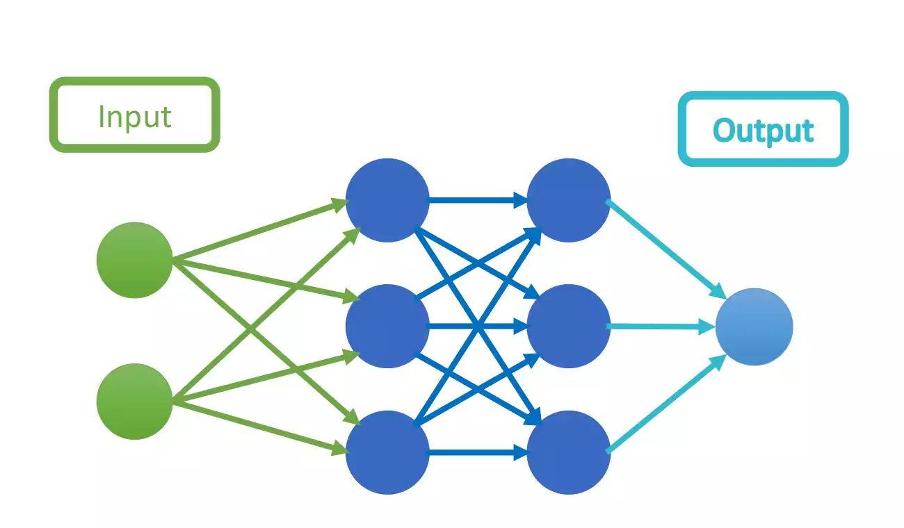
Connectionists Representation.

In the seek for knowledge in SL (in particular on DL), it’s explored ways to interconnect different types of DL architectures in order to solve yet unsolved problems, such as video context awareness classifiers in collision detectors, data fusion and correlation, or even clinical future estimation.

Computer vision has become ubiquitous in our society, with applications in search, image understanding, apps, mapping, medicine, drones, and self-driving cars. Core to many of these applications are visual recognition tasks such as image classification, localization and detection. Recent developments in NN approaches have greatly advanced the performance of these SoA visual recognition systems. This next subsection is a deep dive into details of the DL architectures with a focus on learning end-to-end models and datasets for these tasks, particularly image classification. This part of this documentation, will give detailed resume about neural networks and gain a detailed understanding of cutting-edge research in computer vision that is later reused and applied to create our collision avoidance algorithm.

Deep Learning¶

ANNs were inspired by information processing and distributed communication nodes in biological systems. ANNs have several differences from biological brains. Specifically, neural networks tend to be static and symbolic, while the biological brain of most living organisms is dynamic (plastic) and analog [MWK16, OF96, SB16].

The term DL was introduced to the ML community by Rina Dechter in 1986, [Dec86, Sch15] and to artificial NN by Igor Aizenberg et. al in 2000, in the context of Boolean threshold neurons [AAV01, GS05].

DL is part of a broader family of ML methods based on artificial NN [LBH15b, Sch15].

The first general, working learning algorithm for supervised, deep, feedforward, multilayer perceptrons was published by Alexey Ivakhnenko and Lapa in 1965 [IL65]. A 1971 paper described a deep network with 8 layers trained by the group method of data handling algorithm [Iva71].

The work on DL in computer vision was slightly hibernated, until in 1989, Yann LeCun et al. applied the standard backpropagation algorithm, which had been around as the reverse mode of automatic differentiation since 1970. The impact of DL in industry began in the early 2000s, when CNNs already processed an estimated 10% to 20% of all the checks written in the US [LBH15b].

DL architectures such as deep neural networks, deep belief networks, recurrent neural networks and convolutional neural networks have been applied to fields including computer vision, speech recognition, natural language processing, audio recognition, social network filtering, machine translation, bioinformatics, drug design, medical image analysis, material inspection and board game programs, where they have produced results comparable to and in some cases superior to human experts [AFJ19, ARK10, GLO+16, MSH18, Sch15].

Modern CNNs are considered as one of the best techniques for learning image and video content showing SoA results on image recognition, segmentation, detection, and retrieval related tasks [CGGS12, LDY19]. The success of CNN has captured attention beyond academia. In industry, companies such as Google, Microsoft, AT&T, Facebook and PDM have developed active research groups for exploring new architectures of CNN [DY13].

In DL, each level learns to transform its input data into a slightly more abstract and composite representation. In an image recognition application, the raw input is a matrix of pixels, where the first representational layer may abstract the pixels and encode edges, the second layer may compose and encode arrangements of edges, the third layer may encode a nose and eyes and the fourth layer may recognize that the image contains a face. Moreover, a DL process can learn which features to optimally place in which level on its own [BYC+13, LBH15a].

The deep in deep learning refers to the number of layers through which the data is transformed. More precisely, DL systems have a substantial CAP depth. The CAP is the chain of transformations from input to output. CAPs describe potentially causal connections between input and output. For a feedforward neural network, the depth of the CAPs is that of the network and is the number of hidden layers plus one (as the output layer is also parameterized). For recurrent neural networks, in which a signal may propagate through a layer more than once, the depth is potentially unlimited [Sch15]. No universally agreed upon threshold of depth divides shallow learning from DL, but most researchers agree that DL involves \(depth > 2\). CAP of depth 2 has been shown to be a universal approximator in the sense that it can emulate any function [HOT06]. Beyond that more layers do not add to the function approximator ability of the network. Deep models are able to extract better features than shallow models and hence, extra layers help in learning features.

The DL architectures are often constructed with more layers then the necessary, which helps to disentangle these abstractions and pick out which features improve performance.

CNN topology is divided into multiple learning stages composed of a combination of the convolutional layer, non-linear processing units, and subsampling layers [JKRL09]. As shown in Figure 1.9, the architecture of a typical CNN model is structured as a series of layers. Each layer performs multiple transformations using a bank of convolutional kernels (filters) [LKF10]. All the components involved in such architecture will be later described in section 1.3. Convolution operation extracts locally correlated features by dividing the image into small slices (similar to the retina of the human eye), making it capable of learning suitable features. Output of the convolutional kernels is assigned to non-linear processing units, which not only helps in learning abstraction but also embeds non-linearity in the feature space. The non-linearity outputs different patterns of activations for different responses, which facilitates the learning of semantic in different images. This is usually followed by subsampling, which helps in compressing the results and also makes the input invariant to geometrical distortions [LKF10, SMullerB10].

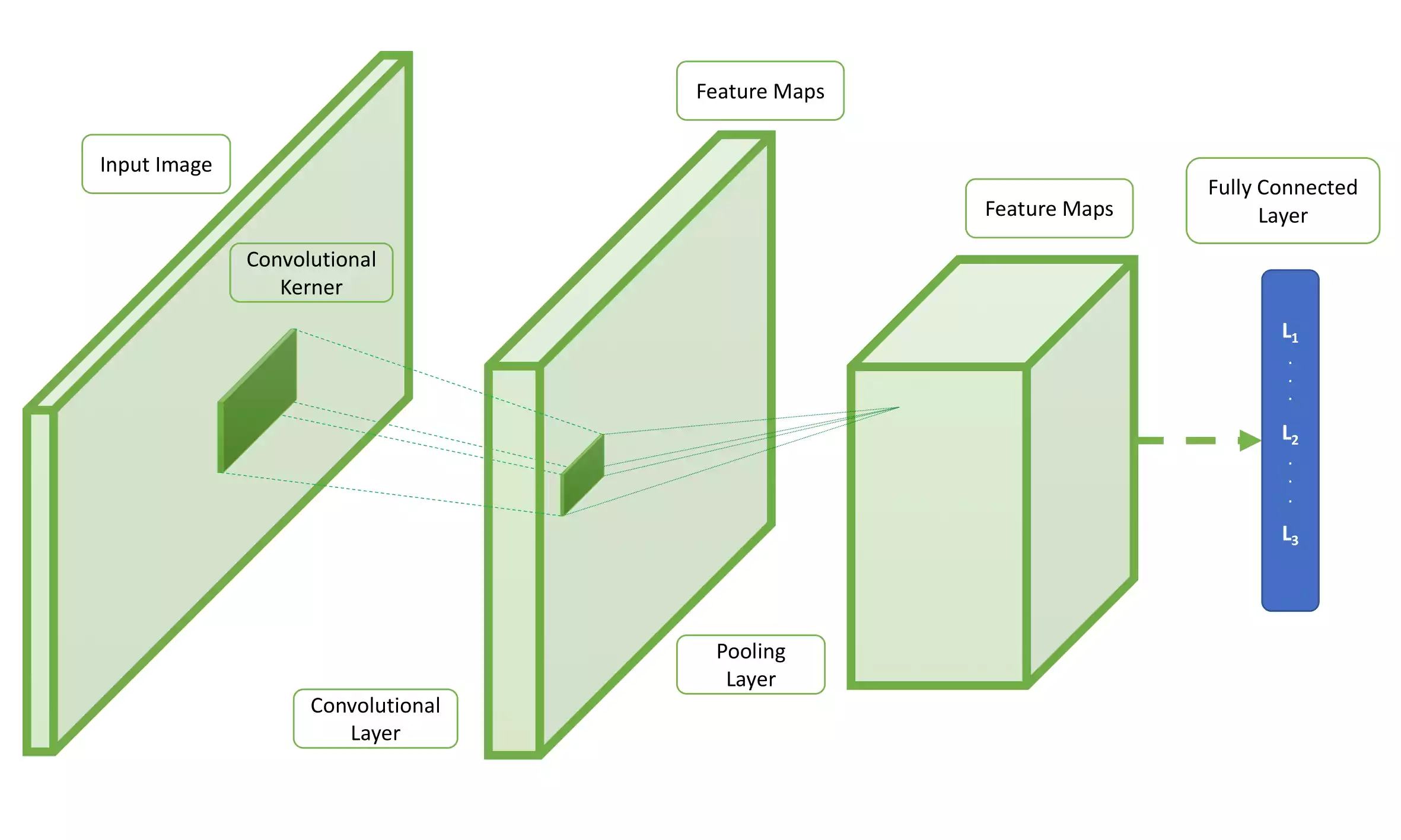
The architecture of a standard Convolutional Neural Network model.

The work conducted by Hubel and Wiesel’s [HW62, HW68] inspired the initial architectural designs of CNNs, following the basic structure of primate’s visual cortex. As illustrated in figure 1.10, the first steps can be considered in 1980, with the initial work in Neocognition like networks [Fuk80]. Using this knowledge, Yann LeCun [LBD+89] proposed a grid-like topological data, which displayed the hierarchical feature extraction ability of CNNs.

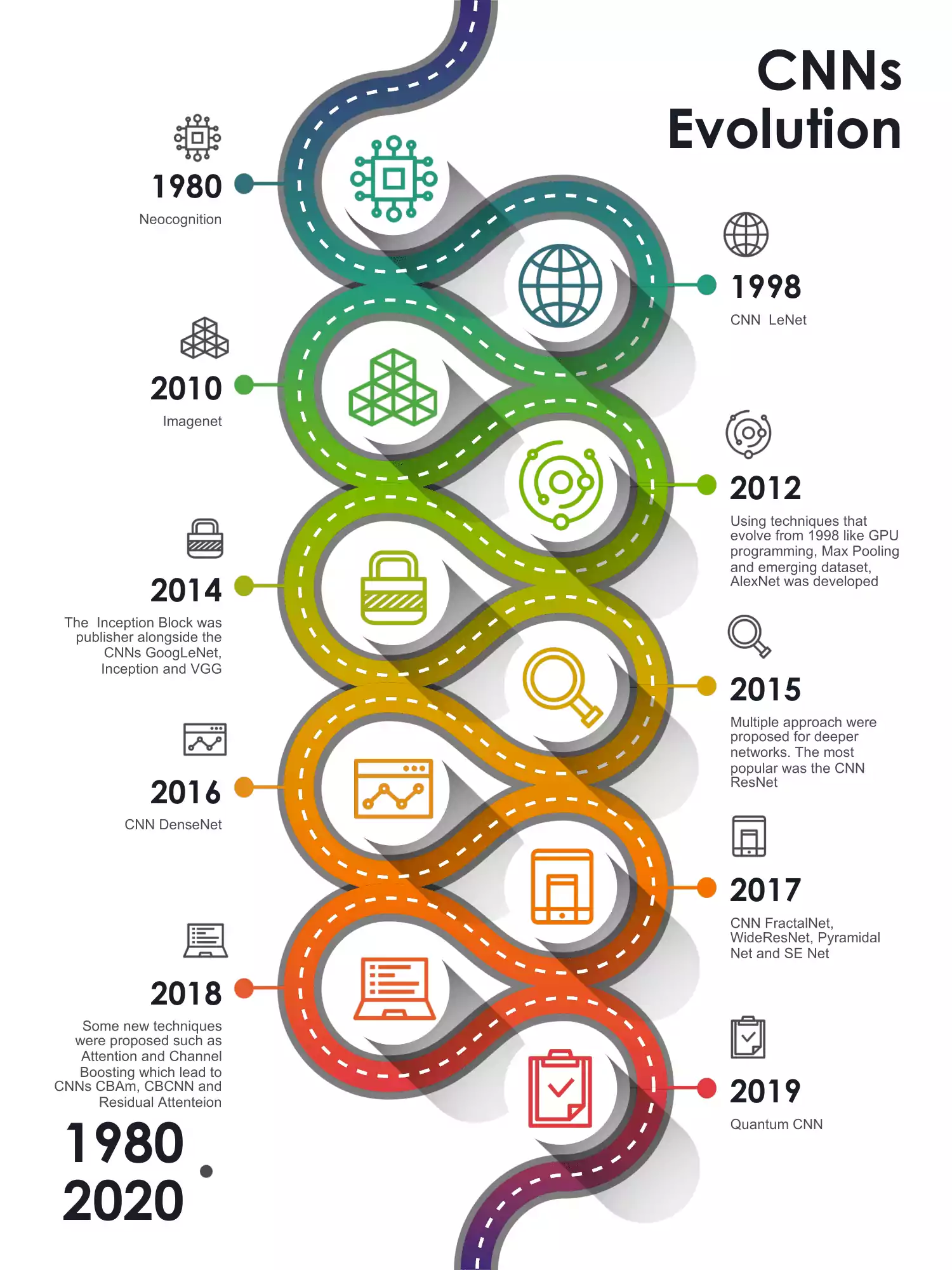
Convolutional Neural Networks evolution over the years.

This hierarchical organization emulates the deep and layered learning process of the Neocortex in the human brain, which extract features from the underlying world [Ben09]. The engineered process in CNN resemblance with V1-V2-V4-IT/VTC primate’s ventral pathway of visual cortex [LGS18]. The retinotopic area provide input to primates visual cortex, where contrast normalization and multi-scale highpass filtering is performed by the lateral geniculate nucleus. Afterwards, different regions of the visual cortex categorized as V1, V2, V3, and V4 classify and detect information. The V1 and V2 areas of the visual cortex can be imagined as the convolutional, and subsampling layers, whereas inferior temporal region are similar to the final layers of CNN, which makes inference about the image [GSWG+18].

CNN training is similar to standard NN, where the weights are regulated with backpropagation algorithm, iterating over multiple input images. In backpropagation, the objective is to minimize a cost function, similar to the response based learning of human brain:cite:p:Najafabadi2015.

The revolution of the use of CNNs for image understating and segmentation occurred when it was discover that the results could be improved by tweaking with layers depth [KSH17]. Deep CNN architectures have advantage over shallow architectures when dealing complex learning problems. Using multiple linear and non-linear neurons in a layer wise mode, enhances this deep networks with the ability to learn representations at different levels of abstraction. Additionally, advances in hardware enabled the renewed the interest. In 2009, Nvidia was involved in what was called the big bang of deep learning, as DNN were trained with Nvidia GPUs [Dix16]. That year, Google Brain used Nvidia GPUs to create capable DNNs. While there, Andrew Ng determined that GPUs could increase the speed of DL systems by about 100 times [TheEconomist10]. In particular, GPUs are well-suited for the matrix/vector math involved in ML [DF17, OJ04]. GPUs speed up training algorithms by orders of magnitude, reducing running times from weeks to days [CMGS10, RMN09]. Specialized hardware and algorithm optimizations can be used for efficient processing [SCYE17].

Significant additional impacts in image or object recognition were noticed from 2011 to 2012. Although CNNs trained by backpropagation had been around for decades, and GPU implementations of NNs for years, including CNNs, fast implementations of CNNs with max-pooling on GPUs in the style of Ciresan and colleagues were needed to progress on computer vision [CMM+11, LBD+08, OJ04].

Image classification was then extended to the more challenging task of generating descriptions (captions) for images, often as a combination of CNNs and LSTMs [FGI+15, VTBE15, ZLL11].

Some researchers assess that the October 2012 ImageNet victory anchored the start of a deep learning revolution that has transformed the AI industry [Met16].

Multiple improvements in CNNs learning strategy and architectures have been presented to make CNNs scalable to large and complex problems. These innovations can be divided as regularization, structural reformulation, parameter optimization and computation efficiency. Major innovations in CNN have been proposed since 2012 and were mainly due to restructuring of processing units and designing of new blocks. Zeiler and Fergus [ZF14] presented the concept of layer-wise visualization of features, which shifted the trend towards features extraction at low spatial resolution in deep architecture such as VGG [SZ15]. Currently, most of the new architectures are built upon the principle of simple and homogeneous topology as it was presented by VGG. However, Google group introduced an interesting idea of split, transform, and merge, which is known as an inception block. The inception block gave the concept of branching within a layer, which allows features abstraction at different spatial scales [SLJ+15]. In 2015, the concept connections skips was introduced by ResNet [HZRS16]. Afterwards, this concept was used by most of the succeeding NN, such as Inception-ResNet, WideResNet and ResNext [SIVA17, XGDollar+17, ZK16].

Towards the improvement of learning capacities of CNNs, different design such as WideResNet, Pyramidal Net, Xception have been proposed, exploring the effect of transformations of additional cardinality and increase in width [HKK17, XGDollar+17, ZK16]. The focus of research moved from parameter optimization and connections optimization towards improved architectural design (layer structure) of the network. This change resulted in many new architectural blocks such as channel boosting, spatial and channel wise exploitation and attention based information processing [KSA18, WJQ+17, WPLK18].

The overfitting problems are raised by the added layers of abstraction, which allow them to model rare dependencies in the training data. Regularization methods such as Ivakhnenko’s unit pruning or weight decay or sparsity can be applied during training to combat overfitting [BYC+13]. Alternatively dropout regularization technique randomly omits neurons from the hidden layers during training. This helps to exclude rare dependencies [DSH13]. Finally, data can be augmented via methods such as cropping and rotating such that smaller training sets can be increased in size to reduce the chances of overfitting, which will be detailed in 1.4.

The learning computation time comes from the many training parameters of the standard DNNs, such as the size (number of layers and number of neurons per layer), the learning rate, and initial weights. Sweeping through the parameter space for optimal parameters may not be feasible due to the cost in time and computational resources. Various tricks, such as batching (computing the gradient on several training examples at once rather than individual examples) [Hin12] speed up computation. Large processing capabilities of many-core architectures (such as GPUs or the specialized CPUs such as Intel Xeon Phi) have produced significant speedups in training, because of the suitability of such processing architectures for the matrix and vector computations [VMPA19, YBuluccD17].

In the recent years, many different surveys were conducted on CNNs that depicted and compared their basic components. The survey reported by Gu [GWK+18] has reviewed the famous models from 2012-2015 along with their core blocks. There are also other similar surveys in literature that discuss different algorithms of CNN and focus on applications for demonstration of results [GLO+16, LKF10, LWL+17, NVK+15, SSM+16]. The following subsections of 1.3 tried to aggregate this information in a concise, yet vast and wide explanation of the field, detailing building blocks, data sets and models.

Basic CNNs Building Blocks¶

For most of the perception applications, CNN is considered as the most widely used ML technique. A typical block diagram of an ML system was shown in Figure 1.9. Since, SoA CNNs possesses both good feature extraction and strong discrimination ability, the most common task are feature extraction and classification.

The most common CNN architecture is composed of alternated layers of convolution and pooling followed by one or two fully connected layers at the end. In some cases, the fully connected layers are swapped with global average pooling layer. In addition to the various learning stages, different regulatory units, such as batch normalization and dropout are also incorporated to optimize CNN performance [Bou06]. The structure of CNNs components play a fundamental role in new architectures designs and thus achieving enhanced performance. This subsection briefly describes and discusses the role of these components in CNN architecture.

Convolutional Layer¶

A convolutional layer (sometimes denominated conv layer) is composed of a set of convolutional kernels (where each neuron act as a kernel). These kernels are linked with a small area of the image known as a receptive field. The image is divided into small blocks (receptive fields) and convoluted with a specific set of weights (multiplying elements of the filter with the corresponding receptive field elements) [Bou06]. This operation have similarities of a convolutional, but they are mathematically different. Convolution layer operation can expressed as follows:

\[C_{l}^{k} = P_{x,y}^{k} * K_{l}^{k} \label{eq:conv_layer}\]

On equation [eq:conv_layer], the input pixel of the image is represented by \(P_{x,y}\), \(x\), \(y\) shows spatial locality and \(K_{l}^{k}\) represents the \(l^{th}\) convolutional kernel of the \(k^{th}\) layer. Dividing the image into small blocks helps extracting local pixel correlations. Different set of features within the image are extracted by sliding convolutional kernel on the whole image with the same set of weights. This weight sharing on the kernels of convolution operation makes CNN parameters efficient when compared to fully connected NN. The convolution operation may further be categorized into different types based on the type and size of filters, type of padding, and the direction of convolution [LBH15b]. If the kernel is symmetric, the convolution operation becomes a correlation operation [GBC16].

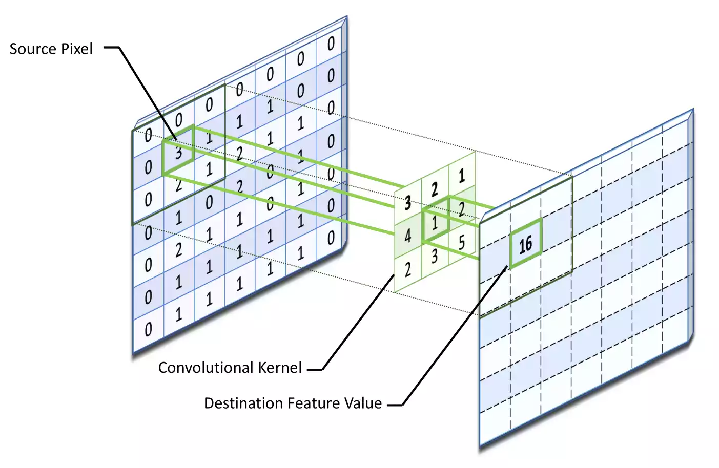
Convolutional layer destination feature value calculation example.

On figure 1.11 is represented an example of the kernel sliding over a source pixel. Initially, the center element of the kernel is placed over the source pixel. Afterwards, the destination pixel, \(C_{l}^{k}\) is then calculated with the weighted sum of itself and nearby pixels. On this example, the resulting destination feature value can be calculated as :

\[C_{l}^{k} = 0*3 + 0*2 + 0*1 + 0*4 + 3*1 + 1*2 + 0*2 + 2*3 + 1*5 = 16 \label{eq:conv_layer_exemple}\]

Pooling Layer¶

The convolution operation outputs feature maps. Once features values are calculated, its exact location becomes less important as long as its approximate position relative to others is preserved. Pooling or downsampling like convolution, is a local operation. It sums up similar information in the neighborhood of the receptive field and outputs the dominant response within this local region [LGT18, LGT16].

On equation [eq:pooling_layer] is represented the pooling operation in which \(Z_{l}\) represents the \(l^{th}\) output feature map, \(C_{x,y}^{l}\) represents the \(l^{th}\) input feature map, whereas \(f_{p}(x)\) defines the type of pooling operation.

\[Z_{l} = f_{p} ( C_{x,y}^{l} ) \label{eq:pooling_layer}\]

The use of pooling operation extracts a combination of features, which are invariant to translational shifts and distortions [RHBL07, SMullerB10]. Reduction in the size of feature map to invariant feature set not only reduces network complexity and also increases generalization by reducing overfitting. The most common types of pooling formulations are [HZRS15, WWCN12]:

Max pooling.
Average pooling.
L2 pooling.
Overlapping pooling.
Spatial pyramid pooling

Activation Function¶

On classification problems, activation functions are used as a decision function, helping to differentiate complex classes. The selection of the activation function can also accelerate the learning process. For CNNs, activation functions of the convolved feature map is defined in equation can be defined as:

\[T_{l}^{k} = f_{A} ( C_{l}^{k} ) \label{eq:activation_layer}\]

On equation [eq:activation_layer], \(C_{l}^{k}\) is the output of a convolution operation, which is mapped to an activation function \(f_{A}(x)\). This activation function adds non-linearity and returns the resulting output \(T_{l}^{k}\) for \(k^{th}\) layer. In academia, different activation functions such as sigmoid, tanh, maxout, ReLU, and variants of ReLU such as leaky ReLU, ELU, and PReLU [LBOMuller12, WJQ+17, WWCN12, XWCL15], are used to inculcate nonlinear combination of features. However, ReLU and its variants are preferred over others activations as it helps in overcoming the vanishing gradient problem [Hoc98, NIGM20].

Many improvements to the learning progress were only possible due to the research of new activation functions. The backpropagation this functions derivatives, so it’s also important to have a clear idea of the activation functions derivatives, because backpropagation is a leaky abstraction (it might use a credit assignment scheme with non-trivial consequences).

Linear¶

The linear activation function, as described in table 1.2, is the most basic activation function. It can be seen as a straight line function where activation is proportional to input (which is the weighted sum from neuron). For the derivative graph, a value of \(m=1\) was considered.

Table 2 Activation Function Linear resume.¶
	Function	Derivative
Formula	\(R(z,m) = z*m\)	\(R'(z,m) = m\)
Python code	def linear(z,m): return m*z	def linear_der(z,m): return (m * z ) / z

The main advantages of using a linear activation function can be described as:

It gives a linear value, for range of activations, which can be used in both regression and classification.
It’s possible to utilize multiple neurons together, and do simple classifications afterwards, such as considering the max value fired.

On the other hand, the linear activation function as some disadvantages, such as:

The derivative is a constant. This has a negative impact on the backpropagation, because the gradient has no relationship with \(x\).
It’s not possible to utilize gradient descent for leaning, because it’s going to be on constant gradient.

ReLU¶

ReLU is the most used activation function in nowadays applications, mainly because the formula is deceptively simple: \(max(0,z)\). Despite its name and appearance, it’s not linear and provides the same benefits as the traditional Sigmoid but with better performance due to it’s computational simplicity. This activation function has been summarized in table 1.3.

Table 3 Activation Function ReLU resume.¶
	Function	Derivative
Formula	\(R(z) = \begin{Bmatrix} z & z > 0 \\ 0 & z <= 0 \end{Bmatrix}\)	\(R'(z) = \begin{Bmatrix} 1 & z>0 0 & z<0 \end{Bmatrix}\)
Python code	def relu(z): return np.where(z >= 0, z, 0)	def relu_der(z): return np.where(z >= 0, 1, 0)

The advantages of using ReLU are quite trivial to understand, but it was a big breakout on the CNNs [WJQ+17, WWCN12, XWCL15]. The main ones can be considered as:

It avoids and rectifies vanishing gradient problem that were present on the antecedent activation functions.
It is less computationally expensive than the tanh and sigmoid because it involves simpler mathematical operations.

Due to its popularity, several researchers have detected some disadvantages in this technique, and have proposed alternative versions [WJQ+17, WWCN12, XWCL15]. Some of these disadvantages are:

The range of ReLU is \([0, \infty]\). This means it has no positive boundary, which makes the classification problem harder, and can force the CNN to overshot.
It should only be used within Hidden layers of a Neural Network Model. There’s no advantage of cropping the negative values in the output layer.
Some gradients can be fragile during training and get discarded. Usually, when this happens, the neuron will update the weights to values which produce negative \(x\) results. When this values are passed to the ReLU it will always returns 0, and due to it’s derivative, it is never again updated, which can be considered a ’dead neuron’.
In another words, f activations in the region \((x<0)\) of ReLU, gradient will be 0 because of which the weights will not get adjusted during descent. That means, those neurons which go into that state will stop responding to variations in error/ input ( simply because gradient is 0, nothing changes ). This is called dying ReLU problem. Some studies conducted to SoA CNN realized that in many architectures, more then 90% of the network is composed of ’dead neuron’ [HPTD15].

ELU¶

The activation function ELU usually converges to zero in a few epoch, which generate fast training and produce more accurate results. Different to other activation functions, ELU uses an \(\alpha\) constant which needs to be positive number. As analyzed in section 1.3.5, ELU is similar to ReLU, except on the negative inputs region. Both functions are a identity function for positive inputs. On the other hand, ELU becomes smooth slowly until its output equal to \(- \alpha\) whereas ReLU swaps to 0 instantaneously, as presented in table 1.4.

Table 4 Activation Function ELU resume.¶
	Function	Derivative
Formula	\(R(z) = \begin{Bmatrix} z & z > 0 \\ \alpha * \left ( e^{z} - 1 \right ) & z <= 0 \end{Bmatrix}\)	\(R'(z) = \begin{Bmatrix} z & z > 0 \\ \alpha * e^{z} & z <= 0 \end{Bmatrix}\)
Python code	def elu(z,alpha): return np.where(z >= 0, z, alpha*(np.exp(z) -1))	def elu_der(z,alpha): return np.where(z >= 0, 1, alpha*np.exp(z))

Some of the benefits of ELU are [XWCL15]:

ELU becomes smooth slowly until its output equal to \(- \alpha\) whereas ReLU sharply smoothes.
ELU is a strong alternative to ReLU.
Unlike to ReLU, ELU can produce negative outputs.

Nonetheless, for \(x > 0\), the ELU activation function can also start overshot with the output range of [0, \(\infty\)] [XWCL15].

LeakyReLU¶

LeakyRelu is yet another variant of ReLU. Instead of being 0 when \(z < 0\), a leaky ReLU allows a narrow, non-zero, constant gradient \(\alpha\) (usually the value \(\alpha = 0.01\) is considered). However, the consistency of the benefit across tasks is presently unclear. This activation function has been summarized in table 1.5. Even thought that usually the value \(\alpha = 0.01\) is considered, for a better graphical representation of the ’leaking’ property, a value of \(\alpha = 0.1\) has been considered.

Table 5 Activation Function LeakyReLU resume.¶
	Function	Derivative
Formula	\(R(z) = \begin{Bmatrix} z & z > 0 \\ \alpha * z & z <= 0 \end{Bmatrix}\)	\(R'(z) = \begin{Bmatrix} 1 & z>0 \\ \alpha & z<0 \end{Bmatrix}\)
Python code	def leakyrelu(z, alpha): return np.where(z >= 0, z, alpha * z)	def leakyrelu_der(z, alpha): return np.where(z>=0, 1, alpha)

Leaky ReLUs are a clear attempt to fix the dead neurons problems of ReLU. By having a narrow negative slope, it allow the gradient to always have an opportunity to train the network, and the possibility to tweak the weights to place it in the positive \(x\) region. Nevertheless, it possess linearity, so it shouldn’t be used for the classification tasks [WJQ+17, WWCN12].

Sigmoid¶

The Sigmoid activation function receives as input a real value and outputs a value between 0 and 1, as can extrapolated from table 1.6. This makes it easy to apply because it contains the most desired proprieties for an activation function. It’s non-linear, continuously differentiable, monotonic, and has a well defined output range [LBOMuller12].

Table 6 Activation Function Sigmoid resume.¶
	Function	Derivative
Formula	\(S(z) = \frac{1} {1 + e^{-z}}\)	\(S'(z) = S(z) \cdot (1 - S(z))\)
Python code	def sigmoid(z): return 1.0 / (1 + np.exp(-z))	def sigmoid_der(z): return sigmoid(z)*(1-sigmoid(z))

The main advantages of the sigmoid function can be described as [LBOMuller12]:

It is nonlinear function, which if combined multiple times, represents a complex output space easier then a linear function.
Produces an analog activation with step function reassembly.
It has a smooth gradient.
The step like shape, gives good results in classification applications.
The output of the activation function is always going to be in range \([0,1]\) compared to \([-\infty, \infty]\) of linear like function. This prevents the output from overshooting.

On the other hand, some disadvantages have been identified by researchers [LBOMuller12], in concrete:

At the extremes of the sigmoid function, the \(y\) values fluctuations are ignored in the \(X\) response.
Also, on the extremes, the gradient tend to 0, which generates the problem of vanishing gradients [Hoc98].
Optimization is not trivial, because the output is not zero centered. On the zero region, the gradient is higher which make the updates flow in different directions.
Random weight initialization, can make the network to refuse to learn drastically slow.

Tanh¶

Tanh activation function is similar to sigmoid, but with the output zero centered, as it is presented in table 1.7. Usually tanh is prefered over sigmoid, due to it’s center [KK92, XHL16].

Table 7 Activation Function Tanh resume.¶
	Function	Derivative
Formula	\(T (z) = \frac{e^{z} - e^ {-z}}{e^{z} + e^{-z}}\)	\(T' (z) = 1 - T(z)^{2}\)
Python code	def tanh(z): return (np.exp(z) - np.exp(-z)) / (np.exp(z) + np.exp(-z))	def tanh_der(z): return 1 - np.power(tanh(z), 2)

Kalman calculated a function based on tanh [KK92]. On his study, he concluded that for deep networks, the gradient is stronger for tanh than sigmoid (due to the derivatives being steeper), which leads to a faster inference. Nonetheless, both sigmoids and tanh don’t address the vanishing gradient problem.

Softmax¶

Finally, the last activation function this dissertation will look into is the Softmax. It calculates the probabilities distribution of the event over \(N\) different events, where the \(N\) is the size of the output array. This function is a quite different from the previous presented in it’s conception. The probabilities of each target class over all possible target classes is calculated utilizing an \(N\) dimensional vector of arbitrary real values and producing another \(N\) dimensional vector with real values in the range \([0, 1]\) that add up to \(1.0\). This is demonstrated in equation [eq:softmaxvectors].

\[\begin{split}\label{eq:softmaxvectors} S(z) : \begin{bmatrix} z_1 \\ z_2 \\ \vdots \\ z_N \end{bmatrix} \rightarrow \begin{bmatrix} S_1 \\ S_2 \\ \vdots \\ S_N \end{bmatrix}\end{split}\]

Since these output are already a probabilities from \([0,1]\), the results can be directly mapped to target classes, and the training not only maximize a value, but also maximize the disparity of triggers.

From a mathematical point of view, where the rest of the functions could be analyzed from a escalar view, softmax is fundamentally a vector function. It takes a vector as input and produces a vector as output. In other words, it has multiple inputs and multiple outputs. Therefore, it’s not possible to represent ’the derivative of softmax’. For this reason, in this activation function is presented more detail.

Since softmax has multiple inputs, with respect to which input element the partial derivative should be computed. Thus, it’s necessary to find the partial derivatives:

\[\label{eq:softmaxder} \frac{\partial S_i}{\partial z_j}\]

This is the partial derivative of the \(i^{th}\) output with respect to the \(j^{th}\) input. A shorter way to write the partial derivative that will be used going forward is \(D_j S_i\). Since softmax is a \(\mathbb{R} ^N \rightarrow \mathbb{R} ^N\) function, the most general derivative computed for it is the Jacobian matrix:

\[\begin{split}\label{eq:softmaxjaco} DS = \begin{bmatrix} D_1 S_1 & \cdots & D_N S_1 \\ \vdots & \ddots & \vdots \\ D_1 S_N& \cdots & D_N S_N \end{bmatrix}\end{split}\]

Computing for arbitrary i and j:

\[\label{eq:softmaxds} D_j S_i = \frac{\partial S_i}{\partial z_j} = \frac{\partial \frac{ e^{z_i}}{\sum_{k=1}^{N} e^{z_k}}}{\partial z_j}\]

Note that no matter which \(z_j\) is yielded, the derivative of the denominator \(\sum_{k=1}^{N} e^{z_k}\), will always yell \(e^{z_j}\). This is not the case for numerator \(e^{z_i}\). The derivative of \(e^{z_i}\) with respect to \(z_j\) is \(e^{z_j}\) only if \(i = j\), because only then \(e^{z_i}\) has \(z_j\) anywhere in it. Otherwise, the derivative is \(0\).

In result, it’s obtained that \(D_j S_i\) can be calculated by:

\[\begin{split}\label{eq:softmaxfder} D_j S_i = \begin{Bmatrix}S_i (1 - S_j) & i = j \\ - S_i S_j & i \neq j\end{Bmatrix}\end{split}\]

In ML literature, the term gradient is commonly used to stand in for the derivative. Gradients are only defined for scalar functions (such as the functions described in the previous sections). For vector functions like softmax it’s imprecise to present it as a gradient. The Jacobian is the fully general derivate of a vector function. Nevertheless, for the sake of coherence, a resume table 1.8 is presented. Keep in mind that both the graphical representation and direct code derivative in Python, the results don’t express much importance. For being a vectorial function, the resulting value \(S(z)\) for a given \(z\) will be highly depend of the number \(N\) of the the \(z\) array, that for this representation \(60\) points from \([-6,6]\) were considered. In practical applications the Jacobian Matrix is calculated, and for graphical representation, the probability of the target class is usually preferred.

Table 8 Activation Function Softmax resume.¶
	Function	Derivative
Formula	\(S ( z_i) = \frac{e^{z_i}}{ \sum_{1}^{j} e^{z_j}}\)	\(S' (z_i) = \begin{Bmatrix}S_i * (1 - S_j) & i = j \\ - S_i * S_j & i \neq j\end{Bmatrix}\)
Python code	def softmax(x): return np.exp(x) / np.sum(np.exp(x), axis=0)	def softmax_der(x): sm = softmax(x) return sm * (1 - sm)

The basic practical difference between Sigmoid and Softmax is that while both give output in \([0,1]\) range, softmax ensures that the sum of outputs along channels (as per specified dimension) is always \(1\), which enables them to be directly mapped to classes probabilities estimation. Sigmoid just makes outputs between \([0,1]\).

Hence, if a one hot encoding scheme is being used, where one channel has probabilities of one class and other channel has probabilities of another, then Softmax activation is preferred.

Batch Normalization¶

Batch normalization is used to address the issues related to internal covariance shift within feature maps. The internal covariance shift is a change in the distribution of hidden units’ values, which slow down the convergence (by forcing learning rate to small value) and requires careful initialization of parameters. Batch normalization for a transformed feature map \(T^{k}_{l}\) can be represented as:

\[N_{l}^{k} = \frac{C_{l}^{k} - \mu _{B} }{ \sqrt{ \sigma _{B}^{2} + \varepsilon } } \label{eq:normalization_layer}\]

In equation [eq:normalization_layer], \(N^{k}_{l}\) represents normalized feature map, \(C^{k}_{l}\) is the input feature map, \(\mu _{B}\) is the mean and \(sigma _{B}^{2}\) depict the variance of a feature map for a mini batch respectively. Batch normalization unifies the distribution of feature map values by bringing them to zero mean and unitary variance [IS15]. Furthermore, it smooths the flow of gradient and acts as a regulating factor, which thus helps in improving generalization of the network.

Dropout¶

The Dropout technique introduces regularization in the network, which ultimately reduces overfitting by randomly skipping some units or connections with a certain probability. In DNNs, multiple connections that learn a non-linear relation are sometimes co-adapted, which reduces generalization [HSK+12]. This random dropping of some connections or units force all neurons to be utilized, by making thinned network architectures trains, and finally one representative network with all weights. This selected architecture is then considered as an approximation of all of the proposed networks [SHK+14].

Fully Connected Layer¶

Fully connected layers are used at the end of the networks for classification or regression purposes. It takes input from the previous layer and globally analyses output of all the preceding layers [LCY14]. This makes a non-linear combination of selected features, which are used for the classification of data [RW17]. For being a process that crosses all values, the number of operations and weights involved usually surpasses the rest of the entire network.

Data Augmentation¶

Data augmentation is an effective technique for improving the accuracy of CNNs [SK19]. Usually Data Augmentations uses transformations such as flipping, color space augmentations, and random cropping. These transformations encode many of the invariance that present challenges to image recognition tasks. Some more advance data augmentations techniques are GAN-based augmentation, neural style transfer, and meta-learning schemes [DT19, KI18]. This section will explain how the common augmentation algorithms works, illustrate experimental results, and discuss disadvantages of the augmentation technique.

Some frameworks such as Keras [Ker19] provide ways to perform Data Augmentation on the fly, rather than performing the operations on your entire image dataset in memory. The API is designed to be iterated by the deep learning model training process, creating augmented image data for the algorithm on run-time. This reduces memory overhead, but adds some additional computation during model training, which result in a longer training time.

In Keras, the IDG calculate the statistics required to actually perform the transforms to the image data. The data generator itself is in fact an iterator, returning batches of image samples when requested. In the most used ML frameworks, when data augmentation is applied, instead of calling the fit function on the model, it’s necessary to call the fit generator function and pass in a IDG with the desired length of an epoch, as well as the total number of epochs on which to train.

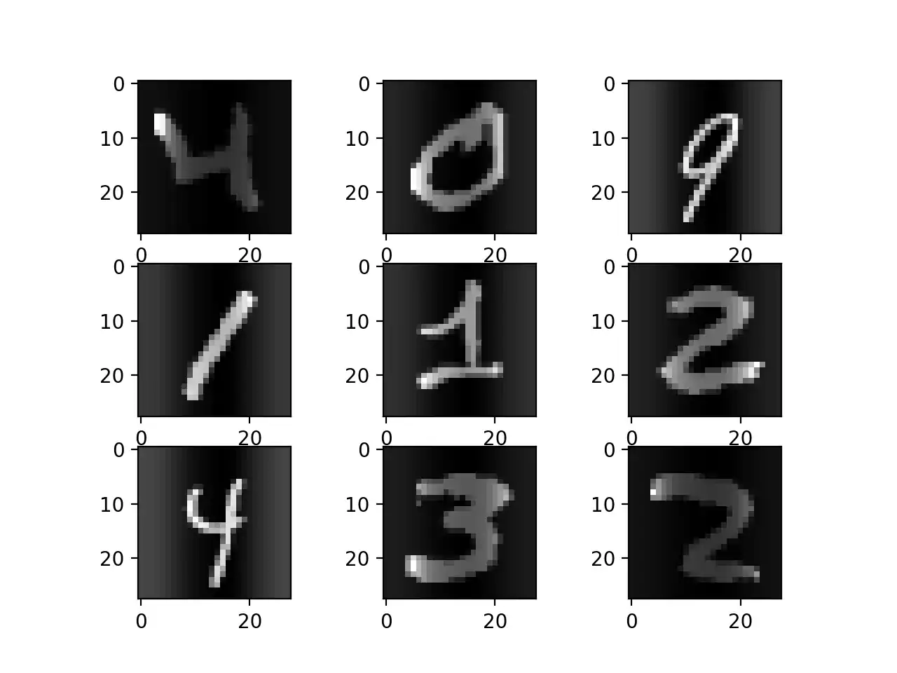
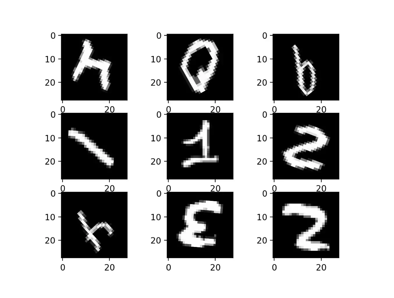
The MNIST dataset [LBBH98] was used in order to have a common set of example images. On figure 1.12 a set of nine images is represented to have a base of comparison for Image Augmentation algorithms.

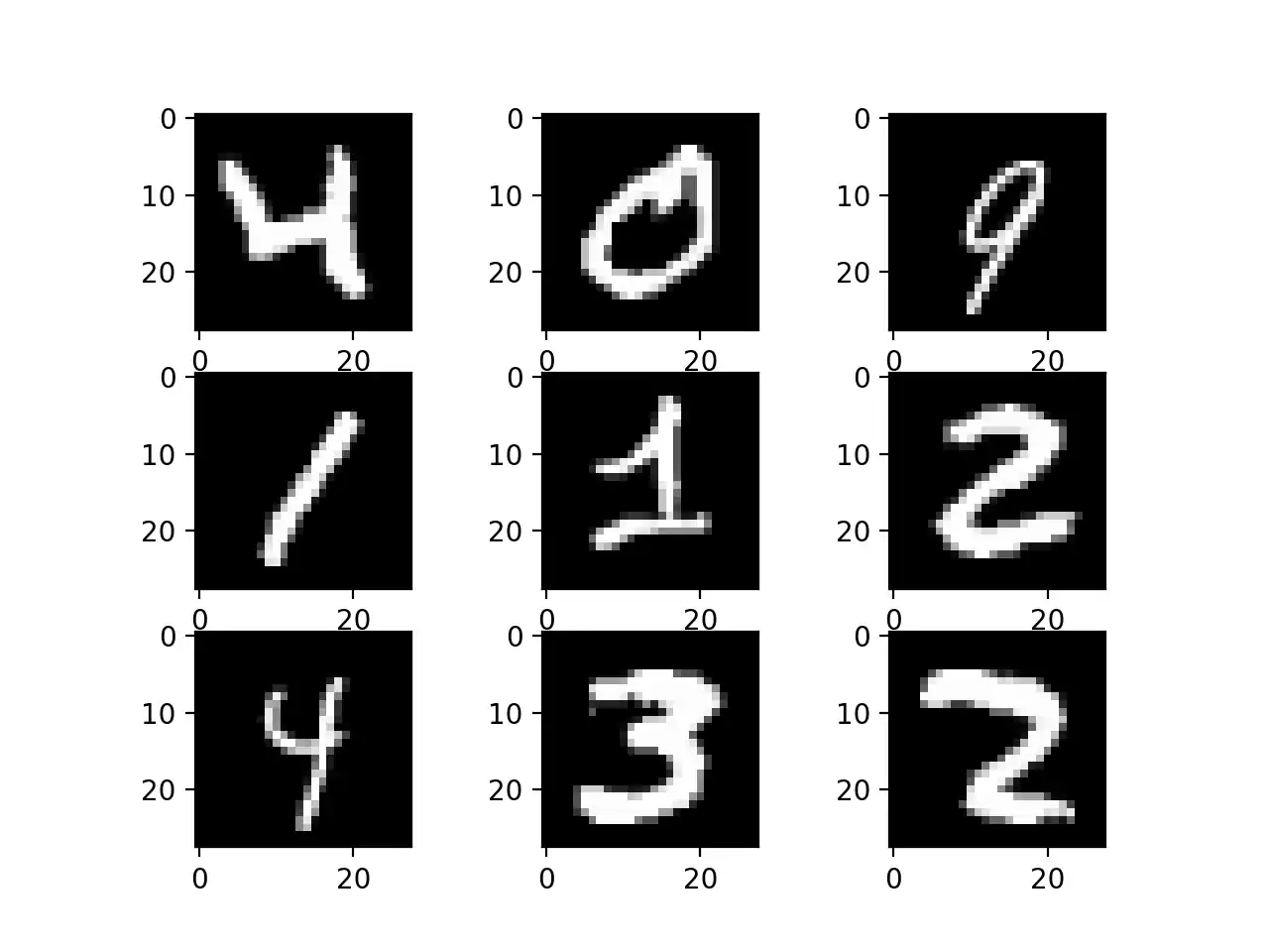
Point Of Comparison.

Feature Standardization¶

Standardization typically means data rescaling, in order to have a mean of \(\mu = 0\) and a standard deviation of \(\sigma =1\) (unit variance). Feature Standardization allows to normalize pixel values across an entire dataset. It mirrors the type of standardization often performed for each column in tabular dataset [SSZ+16]. Usually this is done by performing the equation [eq:features]:

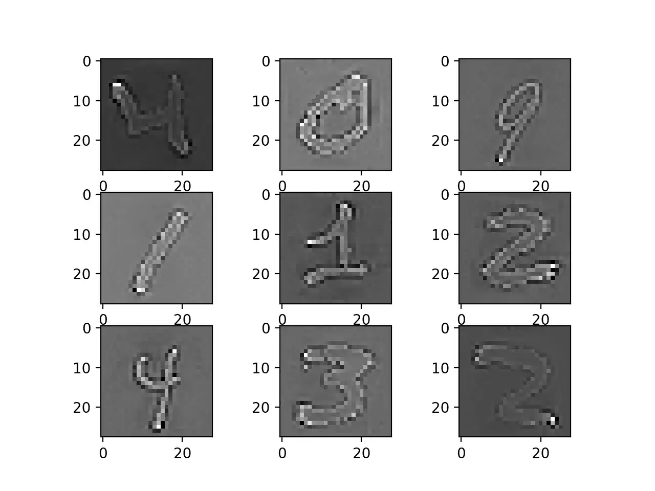
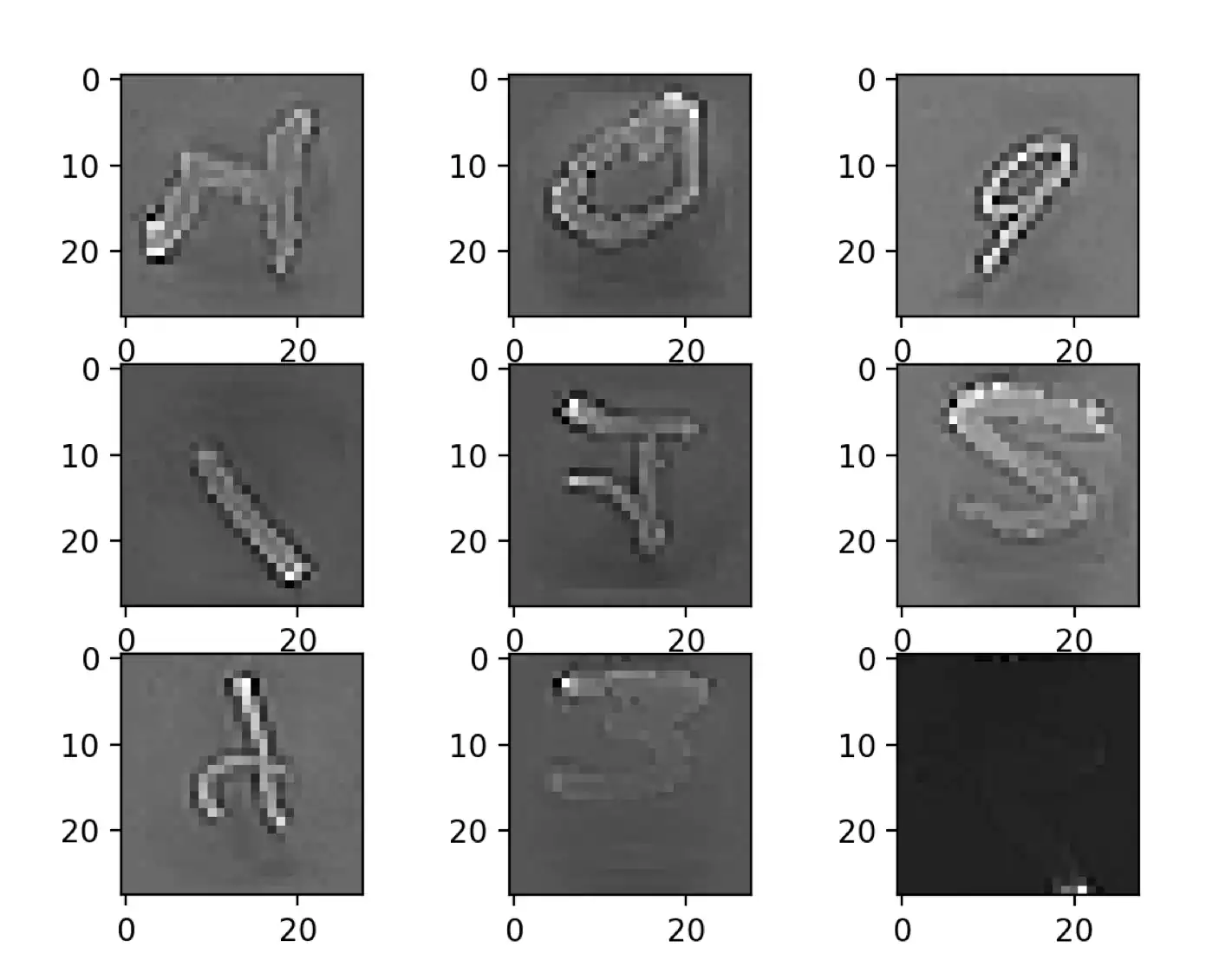
\[\label{eq:features} x' = \frac{x - \bar{x}}{\sigma}\]

On Keras framework, this is achieved by setting the feature-wise center and feature-wise standard normalization arguments on the IDG class. Applying feature standardization on the images of figure 1.12, it’s possible to achieve the result represented on figure 1.13, which result in images seemingly darkening and lightning different digits.

Feature Standardization.

ZCA Whitening¶

A whitening transform of an image is a linear algebra operation that reduces the redundancy in the matrix of pixel images. Less redundancy in the image is intended to better highlight the structures and features in the image to the learning algorithm [LFL15].

Considering \(N\) data point in \(\mathbb{R}^n\), the covariance matrix is \(\Sigma \in \mathbb{R}^{n \times n}\) estimated to be:

\[\label{eq:zcawhiteone} \hat{\Sigma}_{jk} = \frac{1}{N-1} \sum_{i=1}^N (x_{ij} - \bar{x}_j) \cdot (x_{ik} - \bar{x}_k)\]

In equation [eq:zcawhiteone], \(\bar{x}_j\) denotes the \(j^{th}\) component of the estimated mean of the samples \(x\). Any matrix \(W \in \mathbb{R}^{n \times n}\) which satisfies the condition \(W^T W = C^{-1}\) whitens the data. Typically, image whitening is performed using the PCA technique. More recently, an alternative called ZCA shows better results and results in transformed images that keeps all of the original dimensions and unlike PCA, resulting transformed images still look like their originals. To execute a ZCA \(W = M^{- \frac{1}{2}}\).

Using a ZCA Whitening transform on the sample images, the same general structure is maintained and how the outline of each digit is highlighted, as illustrated on 1.14.

ZCA Whitening.

Random Shifts¶

Objects in images may not be centered in the frame. They may be off-center in a variety of different ways. To solve this problem during training, a common technique is to train the deep learning networks to expect and handle off-center objects by artificially creating shifted versions of the training data. For example, Keras and Tensorflow supports separate horizontal and vertical random shifting of training data by the width shift range and height shift range arguments.

Running this example creates shifted versions of the digits, as represented on 1.15. Again, this is not required for MNIST as the handwritten digits are already centered, but it is useful on more complex problem domains.

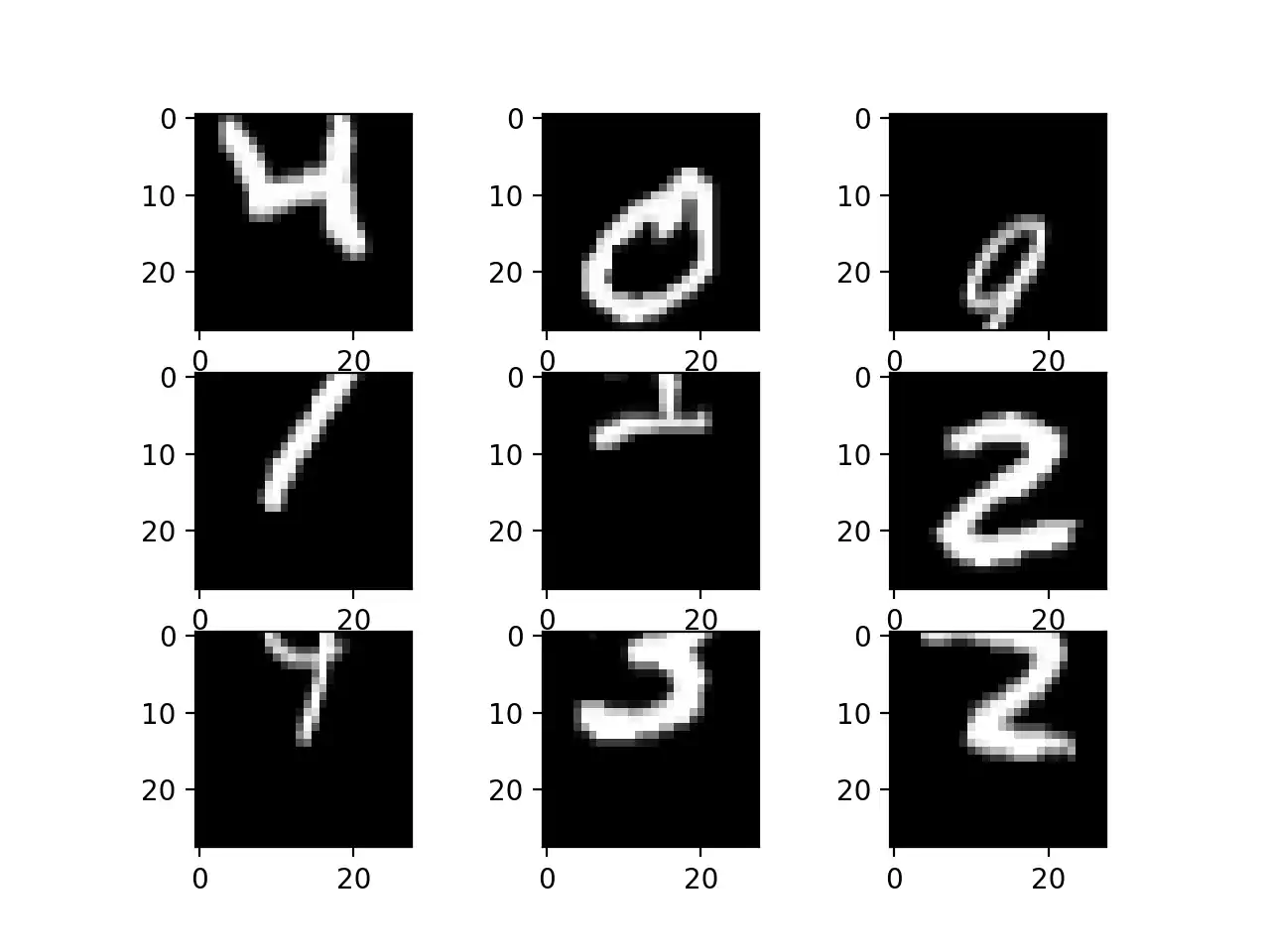
Random Shifts.

Random Flips¶

Another image data augmentation technique that improves the performance is to randomly flip the training images. On figure 1.16 it can be seen it’s result over the sample images. On this example (MNIST dataset), flipping digits is not useful as they require the correct left and right orientation, but this may be useful for images of objects in a scene that can have different orientation.

Random Flips.

Random Rotations¶

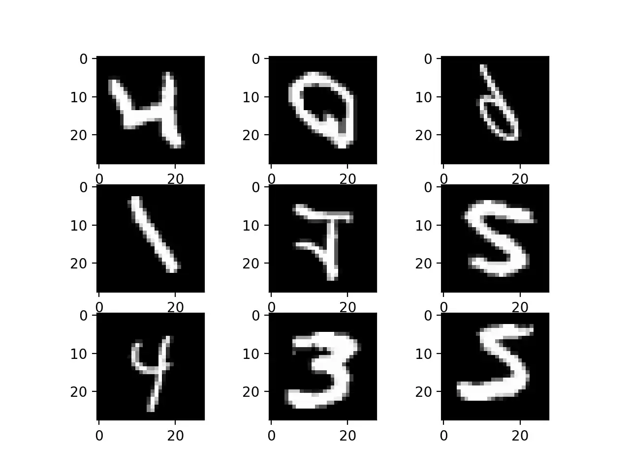
Sometimes images in the dataset may have different rotations in the scene. In those cases, it’s helpful to train the model capable of handling images rotations by artificially and randomly rotating images from the dataset during training.

As seen on figure 1.17 the images have been rotated left and right up to a limit of 180 degrees. This is not helpful on this problem because the MNIST digits have a normalized orientation, but this transform might be of help when learning from photographs where the objects may have different orientations. Not only that but it might to some incorrect labeling. For example, the digit \(9\) at the top right corner is transformed into a \(6\) but will remain labeled as a \(9\) possibly leading to a worse model.

Random Rotations.

Additional Augmentations¶

When doing runtime data augmentations it’s important not to use multiple techniques without a clear idea of the augmented results. As an example of this, it can be observed in figure 1.18 where it was applied random shifts, ZCA whitening, standard normalization, random flips and zoom (between \(\left [ \frac{1}{2}, 2 \right ]\)). It’s questionable if the data represented after augmentation is valid, or if require the model to learn that the number \(2\) is a black square (bottom right image).

Data Augmentation done wrong.

Additionally, some common data augmentations techniques are the rescaling and filling mode. Both this methods are usually applied after the rest of data augmentations techniques. Filling mode can have different flavors points outside the boundaries of the input are filled according to the given mode:

Constant: The outside is filled with a predefined value.

\[\begin{bmatrix}kkkk \left | abcd \right | kkkk \end{bmatrix} (p_val=k)\]
Nearest: The outside is filled with the nearest value of the last pixel.

\[\begin{bmatrix}aaaa \left | abcd \right | dddd \end{bmatrix}\]
Reflect: The outside is filled with a reflection of the values, sometimes called mirror filling.

\[\begin{bmatrix}dcba \left | abcd \right | dcba \end{bmatrix}\]
Wrap: The outside is filled with the opposite values, like the image was a cylinder and the content is wraping around.

\[\begin{bmatrix}abcd \left | abcd \right | abcd \end{bmatrix}\]

Image data is unique in the way that is possible to review the data, create transformed copies and quickly get an idea of how the dataset may be perceive it by the working model. Training DNNs comes with experience, and the quality of the results are interlinked with the tweaks done to the data. For that reason, in conclusion of this page, it’s summarized some tips for getting the most from image data preparation and augmentation for DL.

Review the dataset and do some work with it before starting to train models. In most cases, only a few images actually benefit the training process of your model when augmented, such as the need to handle different shifts, rotations or flips of objects in the scene.
Inspect augmentations. It is one thing to intellectually know what image transforms to use, but in practical cases, it is very different to look at examples results. Reviewing images both with individual augmentations as well as the full set of augmentations planned may unveil ways to simplify or further enhance your model training process.
Lastly, it’s important to evaluate a suite of transforms. Trying more than one image data preparation and augmentation scheme. Often it’s possible that the results of a data preparation scheme are different that what was initially envisioned and the data augmentations are not beneficial.

Bibliography¶

AFJ19: Jamil Ahmad, Haleem Farman, and Zahoor Jan. Deep Learning Methods and Applications. In SpringerBriefs in Computer Science. 2019. doi:10.1007/978-981-13-3459-7_3.
AAV01: I. N. Aizenberg, N. N. Aizenberg, and J. Vandewalle. Multi-Valued and Universal Binary Neurons: Theory, Learning, and Applications. IEEE Transactions on Neural Networks, 2001. doi:10.1109/TNN.2001.925572.
ARK10: Itamar Arel, Derek Rose, and Thomas Karnowski. Deep machine learning-A new frontier in artificial intelligence research. IEEE Computational Intelligence Magazine, 2010. doi:10.1109/MCI.2010.938364.
Ayo10: Taiwo Oladipupo Ayodele. Types of Machine Learning Algorithms. New Advances in Machine Learning, 2010. doi:10.5772/56672.
BYC+13(1,2): Bengio, Yoshua, Courville, Aaron, Vincent, and Pascal. Representation learning: A review and new perspectives. IEEE Transactions on Pattern Analysis and Machine Intelligence, 2013. doi:10.1109/TPAMI.2013.50.
Ben09: Y. Bengio. Learning Deep Architectures for AI. Foundations and Trends® in Machine Learning, 2009. doi:10.1561/2200000006.
Bou06(1,2): Jake Bouvrie. Notes on convolutional neural networks. 2006. Online; accessed 01 July 2019. URL: http://cogprints.org/5869/, arXiv:1102.0183, doi:http://dx.doi.org/10.1016/j.protcy.2014.09.007.
CT10: Gavin C. Cawley and Nicola L.C. Talbot. On over-fitting in model selection and subsequent selection bias in performance evaluation. Journal of Machine Learning Research, 2010.
CGGS12: Dan C. Cireşan, Alessandro Giusti, Luca M. Gambardella, and Jürgen Schmidhuber. Deep neural networks segment neuronal membranes in electron microscopy images. In Advances in Neural Information Processing Systems. 2012.
CMM+11: Dan C. Cireşan, Ueli Meier, Jonathan Masci, Luca M. Gambardella, and Jürgen Schmidhuber. Flexible, high performance convolutional neural networks for image classification. In IJCAI International Joint Conference on Artificial Intelligence. 2011. doi:10.5591/978-1-57735-516-8/IJCAI11-210.
CMGS10: Dan Claudiu Cireşan, Ueli Meier, Luca Maria Gambardella, and Jürgen Schmidhuber. Deep, big, simple neural nets for handwritten digit recognition. In IEEE Neural Computation, volume 22, 3207–3220. MIT Press, 2010. doi:10.1162/NECO_a_00052.
CV95: Corinna Cortes and Vladimir Vapnik. Support-Vector Networks. Machine Learning, 1995. doi:10.1023/A:1022627411411.
DSH13: George E. Dahl, Tara N. Sainath, and Geoffrey E. Hinton. Improving deep neural networks for LVCSR using rectified linear units and dropout. In ICASSP, IEEE International Conference on Acoustics, Speech and Signal Processing - Proceedings. 2013. doi:10.1109/ICASSP.2013.6639346.
DF17: Darmatasia and Mohamad Ivan Fanany. Handwriting recognition on form document using convolutional neural network and support vector machines (CNN-SVM). In 2017 5th International Conference on Information and Communication Technology, ICoIC7 2017. 2017. doi:10.1109/ICoICT.2017.8074699.
Dar18: Ashraf Darwish. Bio-inspired computing: Algorithms review, deep analysis, and the scope of applications. Future Computing and Informatics Journal, 2018. doi:10.1016/j.fcij.2018.06.001.
Dec86: Rina Dechter. Learning While Searching in Constraint-Satisfaction-Problems. Aaai, 1986.
DRT11: Houtao Deng, George Runger, and Eugene Tuv. Bias of importance measures for multi-valued attributes and solutions. In Lecture Notes in Computer Science (including subseries Lecture Notes in Artificial Intelligence and Lecture Notes in Bioinformatics). 2011. doi:10.1007/978-3-642-21738-8_38.
DY13: Li Deng and Dong Yu. Deep Learning: Methods and Applications Foundations and Trends R in Signal Processing. Signal Processing, 2013. arXiv:1309.1501, doi:10.1561/2000000039.
DT19: Terrance DeVries and Graham W. Taylor. Dataset augmentation in feature space. In 5th International Conference on Learning Representations, ICLR 2017 - Workshop Track Proceedings. 2019. arXiv:1702.05538.
Dix16: Chris Dixon. What's next in computing? 2016. Online; accessed 4 June 2019. URL: https://www.medium.com.
Dom12(1,2): Pedro Domingos. A few useful things to know about machine learning. In Communications of the ACM. 2012. doi:10.1145/2347736.2347755.
Dom15(1,2): Pedro Domingos. The Master Algorithm. Penguin Books, 2017 edition, 2015. ISBN 9780141979243.
FGI+15: Hao Fang, Saurabh Gupta, Forrest Iandola, Rupesh K. Srivastava, Li Deng, Piotr Dollár, Jianfeng Gao, Xiaodong He, Margaret Mitchell, John C. Platt, C. Lawrence Zitnick, and Geoffrey Zweig. From captions to visual concepts and back. In Proceedings of the IEEE Computer Society Conference on Computer Vision and Pattern Recognition. 2015. doi:10.1109/CVPR.2015.7298754.
Fuk80: Kunihiko Fukushima. Neocognition: a self. In Biol. Cybernetics. 1980. arXiv:arXiv:1011.1669v3, doi:10.1007/BF00344251.
GS05: Faustino J. Gomez and Jürgen Schmidhuber. Co-evolving recurrent neurons learn deep memory POMDPs. In GECCO '05: Proceedings of the 7th annual conference on Genetic and evolutionary computation, 491–498. June 2005. doi:10.1145/1068009.1068092.
GBC16: Ian Goodfellow, Yoshua Bengio, and Aaron Courville. Deep Learning. MIT Press, 2016. ISBN 3540620583, 9783540620587. URL: http://www.deeplearningbook.org, arXiv:arXiv:1011.1669v3, doi:10.1016/B978-0-12-391420-0.09987-X.
GSWG+18: Kalanit Grill-Spector, Kevin S. Weiner, Jesse Gomez, Anthony Stigliani, and Vaidehi S. Natu. The functional neuroanatomy of face perception: From brain measurements to deep neural networks. Interface Focus, 2018. doi:10.1098/rsfs.2018.0013.
GWK+18: Jiuxiang Gu, Zhenhua Wang, Jason Kuen, Lianyang Ma, Amir Shahroudy, Bing Shuai, Ting Liu, Xingxing Wang, Gang Wang, Jianfei Cai, and Tsuhan Chen. Recent advances in convolutional neural networks. Pattern Recognition, 2018. doi:10.1016/j.patcog.2017.10.013.
GLO+16(1,2): Yanming Guo, Yu Liu, Ard Oerlemans, Songyang Lao, Song Wu, and Michael S. Lew. Deep learning for visual understanding: A review. Neurocomputing, 2016. doi:10.1016/j.neucom.2015.09.116.
HKK17: Dongyoon Han, Jiwhan Kim, and Junmo Kim. Deep pyramidal residual networks. In Proceedings - 30th IEEE Conference on Computer Vision and Pattern Recognition, CVPR 2017. 2017. arXiv:1610.02915, doi:10.1109/CVPR.2017.668.
HPTD15: Song Han, Jeff Pool, John Tran, and William Dally. Learning both weights and connections for efficient neural network. In C. Cortes, N. D. Lawrence, D. D. Lee, M. Sugiyama, and R. Garnett, editors, Advances in Neural Information Processing Systems 28, pages 1135–1143. Curran Associates, Inc., 2015. URL: http://papers.nips.cc/paper/5784-learning-both-weights-and-connections-for-efficient-neural-network.pdf.
HZRS15: Kaiming He, Xiangyu Zhang, Shaoqing Ren, and Jian Sun. Spatial Pyramid Pooling in Deep Convolutional Networks for Visual Recognition. IEEE Transactions on Pattern Analysis and Machine Intelligence, 2015. doi:10.1109/TPAMI.2015.2389824.
HZRS16: Kaiming He, Xiangyu Zhang, Shaoqing Ren, and Jian Sun. Deep residual learning for image recognition. In Proceedings of the IEEE Computer Society Conference on Computer Vision and Pattern Recognition. 2016. arXiv:1512.03385, doi:10.1109/CVPR.2016.90.
Hin12: Geoffrey E. Hinton. A practical guide to training restricted boltzmann machines. Lecture Notes in Computer Science (including subseries Lecture Notes in Artificial Intelligence and Lecture Notes in Bioinformatics), 2012. doi:10.1007/978-3-642-35289-8-32.
HOT06: Geoffrey E. Hinton, Simon Osindero, and Yee Whye Teh. A fast learning algorithm for deep belief nets. Neural Computation, 2006. doi:10.1162/neco.2006.18.7.1527.
HSK+12: Geoffrey E. Hinton, Nitish Srivastava, Alex Krizhevsky, Ilya Sutskever, and Ruslan R. Salakhutdinov. Improving neural networks by preventing co-adaptation of feature detectors. CoRR, 2012. URL: http://arxiv.org/abs/1207.0580, arXiv:1207.0580.
Hoc98(1,2): Sepp Hochreiter. The vanishing gradient problem during learning recurrent neural nets and problem solutions. International Journal of Uncertainty, Fuzziness and Knowlege-Based Systems, 1998. doi:10.1142/S0218488598000094.
HW62: D. H. Hubel and T. N. Wiesel. Receptive fields, binocular interaction and functional architecture in the cat's visual cortex. The Journal of Physiology, 1962. doi:10.1113/jphysiol.1962.sp006837.
HW68: D. H. Hubel and T. N. Wiesel. Receptive fields and functional architecture of monkey striate cortex. The Journal of Physiology, 1968. doi:10.1113/jphysiol.1968.sp008455.
IS15: Sergey Ioffe and Christian Szegedy. Batch normalization: Accelerating deep network training by reducing internal covariate shift. In 32nd International Conference on Machine Learning, ICML 2015. 2015. arXiv:1502.03167.
Iva71: A. G. Ivakhnenko. Polynomial Theory of Complex Systems. IEEE Transactions on Systems, Man and Cybernetics, 1971. doi:10.1109/TSMC.1971.4308320.
IL65: A. G. Ivakhnenko and V. G. Lapa. Cybernetic predicting devices. In CCM Information Corporation. 1965.
JKRL09: Kevin Jarrett, Koray Kavukcuoglu, Marc'Aurelio Ranzato, and Yann LeCun. What is the best multi-stage architecture for object recognition? In Proceedings of the IEEE International Conference on Computer Vision. 2009. doi:10.1109/ICCV.2009.5459469.
KK92(1,2): B.L. Kalman and S.C. Kwasny. Why tanh: choosing a sigmoidal function. In [Proceedings 1992] IJCNN International Joint Conference on Neural Networks, volume 4, 578–581 vol.4. 1992. doi:10.1109/IJCNN.1992.227257.
KaminskiJS18: Bogumił Kamiński, Michał Jakubczyk, and Przemysław Szufel. A framework for sensitivity analysis of decision trees. Central European Journal of Operations Research, 2018. doi:10.1007/s10100-017-0479-6.
KSO94: A. W. Kemp, A. Stuart, and J. K. Ord. Kendall's Advanced Theory of Statistics. The Statistician, 1994. doi:10.2307/2348968.
Ker19: Keras. Keras Image Preprocessing. 2019. Online; accessed 01 July 2019. URL: https://keras.io/preprocessing/image/.
KSA18: missing booktitle in khan2018new
KI18: Tomohiko Konno and Michiaki Iwazume. Icing on the cake: an easy and quick post-learnig method you can try after deep learning. arXiv, 2018. arXiv:1807.06540.
KSH17: Alex Krizhevsky, Ilya Sutskever, and Geoffrey E. Hinton. ImageNet classification with deep convolutional neural networks. Communications of the ACM, 2017. doi:10.1145/3065386.
LGS18: missing booktitle in laskar2018correspondence
LBD+89: Y. LeCun, B. Boser, J. S. Denker, D. Henderson, R. E. Howard, W. Hubbard, and L. D. Jackel. Backpropagation Applied to Handwritten Zip Code Recognition. IEEE Neural Computation, 1989. doi:10.1162/neco.1989.1.4.541.
LBD+08: Y. LeCun, B. Boser, J. S. Denker, D. Henderson, R. E. Howard, W. Hubbard, and L. D. Jackel. Backpropagation Applied to Handwritten Zip Code Recognition. IEEE Neural Computation, 2008. doi:10.1162/neco.1989.1.4.541.
LBH15a: Yann Lecun, Yoshua Bengio, and Geoffrey Hinton. Deep Learning (Tutorial Slides). Advances in Neural Information Processing Systems 28 (NIPS 2015), 2015. arXiv:arXiv:1312.6184v5, doi:10.1038/nature14539.
LBH15b(1,2,3): Yann Lecun, Yoshua Bengio, and Geoffrey Hinton. Deep learning. In Nature. 2015. doi:10.1038/nature14539.
LBBH98: Yann LeCun, Léon Bottou, Yoshua Bengio, and Patrick Haffner. Gradient-based learning applied to document recognition. Proceedings of the IEEE, 1998. doi:10.1109/5.726791.
LKF10(1,2,3): Yann LeCun, Koray Kavukcuoglu, and Clément Farabet. Convolutional networks and applications in vision. In ISCAS 2010 - 2010 IEEE International Symposium on Circuits and Systems: Nano-Bio Circuit Fabrics and Systems. 2010. doi:10.1109/ISCAS.2010.5537907.
LBOMuller12(1,2,3,4): Yann A. LeCun, Léon Bottou, Genevieve B. Orr, and Klaus Robert Müller. Efficient backprop. Lecture Notes in Computer Science (including subseries Lecture Notes in Artificial Intelligence and Lecture Notes in Bioinformatics), 2012. doi:10.1007/978-3-642-35289-8-3.
LGT18: Chen Yu Lee, Patrick Gallagher, and Zhuowen Tu. Generalizing Pooling Functions in CNNs: Mixed, Gated, and Tree. IEEE Transactions on Pattern Analysis and Machine Intelligence, 2018. doi:10.1109/TPAMI.2017.2703082.
LGT16: Chen Yu Lee, Patrick W. Gallagher, and Zhuowen Tu. Generalizing pooling functions in convolutional neural networks: Mixed, gated, and tree. In Proceedings of the 19th International Conference on Artificial Intelligence and Statistics, AISTATS 2016. 2016. arXiv:1509.08985.
LFL15: Zuhe Li, Yangyu Fan, and Weihua Liu. The effect of whitening transformation on pooling operations in convolutional autoencoders. Eurasip Journal on Advances in Signal Processing, 2015. doi:10.1186/s13634-015-0222-1.
LCY14: Min Lin, Qiang Chen, and Shuicheng Yan. Network in network. In 2nd International Conference on Learning Representations, ICLR 2014 - Conference Track Proceedings. 2014. arXiv:1312.4400.
LWL+17: Weibo Liu, Zidong Wang, Xiaohui Liu, Nianyin Zeng, Yurong Liu, and Fuad E. Alsaadi. A survey of deep neural network architectures and their applications. Neurocomputing, 2017. doi:10.1016/j.neucom.2016.12.038.
LDY19: Xiaolong Liu, Zhidong Deng, and Yuhan Yang. Recent progress in semantic image segmentation. Artificial Intelligence Review, 2019. doi:10.1007/s10462-018-9641-3.
MWK16: Adam H. Marblestone, Greg Wayne, and Konrad P. Kording. Toward an Integration of Deep Learning and Neuroscience. Frontiers in Computational Neuroscience, 2016. doi:10.3389/fncom.2016.00094.
Met16: Justin Metz. The AI Revolution: Why Deep Learning Is Suddenly Changing Your Life. 2016. Online; accessed 20 April 2020. URL: https://fortune.com/.
MSH18: Seyed Sajad Mousavi, Michael Schukat, and Enda Howley. Deep Reinforcement Learning: An Overview. In Lecture Notes in Networks and Systems. 2018. doi:10.1007/978-3-319-56991-8_32.
NVK+15: Maryam M. Najafabadi, Flavio Villanustre, Taghi M. Khoshgoftaar, Naeem Seliya, Randall Wald, and Edin Muharemagic. Deep learning applications and challenges in big data analytics. Journal of Big Data, 2015. doi:10.1186/s40537-014-0007-7.
NIGM20: Chigozie Nwankpa, Winifred Ijomah, Anthony Gachagan, and Stephen Marshall. Activation functions: comparison of trends in practice and research for deep learning. In Conference: 2nd International Conference on Computational Sciences and Technology, (INCCST) 2020. 2020. arXiv:1811.03378.
OJ04(1,2): Kyoung Su Oh and Keechul Jung. GPU implementation of neural networks. Pattern Recognition, 2004. doi:10.1016/j.patcog.2004.01.013.
OF96: Bruno A. Olshausen and David J. Field. Emergence of simple-cell receptive field properties by learning a sparse code for natural images. Nature, 1996. doi:10.1038/381607a0.
RMN09: Rajat Raina, Anand Madhavan, and Andrew Y. Ng. Large-scale deep unsupervised learning using graphics processors. In Proceedings of the 26th Annual International Conference on Machine Learning. June 2009. doi:10.1145/1553374.1553486.
RHBL07: Marc'Aurelio Ranzato, Fu Jie Huang, Y. Lan Boureau, and Yann LeCun. Unsupervised learning of invariant feature hierarchies with applications to object recognition. In Proceedings of the IEEE Computer Society Conference on Computer Vision and Pattern Recognition. 2007. doi:10.1109/CVPR.2007.383157.
RW17: Waseem Rawat and Zenghui Wang. Deep convolutional neural networks for image classification: A comprehensive review. In IEEE Neural Computation. 2017. doi:10.1162/NECO_a_00990.
SB16: Benjamin Scellier and Yoshua Bengio. Towards a Biologically Plausible Backprop. Arxiv, 2016. arXiv:1602.05179.
SMullerB10(1,2): Dominik Scherer, Andreas Müller, and Sven Behnke. Evaluation of pooling operations in convolutional architectures for object recognition. In Lecture Notes in Computer Science (including subseries Lecture Notes in Artificial Intelligence and Lecture Notes in Bioinformatics). 2010. doi:10.1007/978-3-642-15825-4_10.
Sch15(1,2,3,4): Jürgen Schmidhuber. Deep Learning in neural networks: An overview. 2015. doi:10.1016/j.neunet.2014.09.003.
SSZ+16: Fumin Shen, Chunhua Shen, Xiang Zhou, Yang Yang, and Heng Tao Shen. Face image classification by pooling raw features. Pattern Recognition, 2016. arXiv:1406.6811, doi:10.1016/j.patcog.2016.01.010.
SK19: Connor Shorten and Taghi M. Khoshgoftaar. A survey on Image Data Augmentation for Deep Learning. Journal of Big Data, 2019. doi:10.1186/s40537-019-0197-0.
SZ15: Karen Simonyan and Andrew Zisserman. Very deep convolutional networks for large-scale image recognition. In 3rd International Conference on Learning Representations, ICLR 2015 - Conference Track Proceedings. 2015. arXiv:1409.1556.
SSM+16: Suraj Srinivas, Ravi Kiran Sarvadevabhatla, Konda Reddy Mopuri, Nikita Prabhu, Srinivas S.S. Kruthiventi, and R. Venkatesh Babu. A taxonomy of deep convolutional neural nets for computer vision. Frontiers Robotics AI, 2016. arXiv:1601.06615, doi:10.3389/frobt.2015.00036.
SHK+14: Nitish Srivastava, Geoffrey Hinton, Alex Krizhevsky, Ilya Sutskever, and Ruslan Salakhutdinov. Dropout: A simple way to prevent neural networks from overfitting. Journal of Machine Learning Research, 2014.
SAHG11: Alexander Statnikov, Constantin F Aliferis, Douglas P Hardin, and Isabelle Guyon. Support Vector Clustering. In A Gentle Introduction to Support Vector Machines in Biomedicine. 2011. doi:10.1142/9789814335140_0009.
SCYE17: Vivienne Sze, Yu Hsin Chen, Tien Ju Yang, and Joel S. Emer. Efficient Processing of Deep Neural Networks: A Tutorial and Survey. In Proceedings of the IEEE. 2017. doi:10.1109/JPROC.2017.2761740.
SIVA17: Christian Szegedy, Sergey Ioffe, Vincent Vanhoucke, and Alexander A. Alemi. Inception-v4, inception-ResNet and the impact of residual connections on learning. In 31st AAAI Conference on Artificial Intelligence, AAAI 2017. 2017. arXiv:1602.07261.
SLJ+15: Christian Szegedy, Wei Liu, Yangqing Jia, Pierre Sermanet, Scott Reed, Dragomir Anguelov, Dumitru Erhan, Vincent Vanhoucke, and Andrew Rabinovich. Going deeper with convolutions. In Proceedings of the IEEE Computer Society Conference on Computer Vision and Pattern Recognition. 2015. arXiv:1409.4842, doi:10.1109/CVPR.2015.7298594.
VMPA19: André Viebke, Suejb Memeti, Sabri Pllana, and Ajith Abraham. CHAOS: a parallelization scheme for training convolutional neural networks on Intel Xeon Phi. Journal of Supercomputing, 2019. doi:10.1007/s11227-017-1994-x.
VTBE15: Oriol Vinyals, Alexander Toshev, Samy Bengio, and Dumitru Erhan. Show and tell: A neural image caption generator. In Proceedings of the IEEE Computer Society Conference on Computer Vision and Pattern Recognition. 2015. doi:10.1109/CVPR.2015.7298935.
WJQ+17(1,2,3,4,5): Fei Wang, Mengqing Jiang, Chen Qian, Shuo Yang, Cheng Li, Honggang Zhang, Xiaogang Wang, and Xiaoou Tang. Residual attention network for image classification. In Proceedings - 30th IEEE Conference on Computer Vision and Pattern Recognition, CVPR 2017. 2017. arXiv:1704.06904, doi:10.1109/CVPR.2017.683.
WWCN12(1,2,3,4,5): Tao Wang, David J. Wu, Adam Coates, and Andrew Y. Ng. End-to-end text recognition with convolutional neural networks. In Proceedings - International Conference on Pattern Recognition. 2012.
WPLK18: Sanghyun Woo, Jongchan Park, Joon Young Lee, and In So Kweon. CBAM: Convolutional block attention module. In Lecture Notes in Computer Science (including subseries Lecture Notes in Artificial Intelligence and Lecture Notes in Bioinformatics). 2018. arXiv:1807.06521, doi:10.1007/978-3-030-01234-2_1.
XGDollar+17(1,2): Saining Xie, Ross Girshick, Piotr Dollár, Zhuowen Tu, and Kaiming He. Aggregated residual transformations for deep neural networks. In Proceedings - 30th IEEE Conference on Computer Vision and Pattern Recognition, CVPR 2017. 2017. arXiv:1611.05431, doi:10.1109/CVPR.2017.634.
XHL16: Bing Xu, Ruitong Huang, and Mu Li. Revise saturated activation functions. 2016. arXiv:1602.05980.
XWCL15(1,2,3,4,5): Bing Xu, Naiyan Wang, Tianqi Chen, and Mu Li. Empirical evaluation of rectified activations in convolutional network. CoRR, 2015. URL: http://arxiv.org/abs/1505.00853, arXiv:1505.00853.
YBuluccD17: Yang You, Aydın Buluç, and James Demmel. Scaling deep learning on GPU and knights landing clusters. In Proceedings of the International Conference for High Performance Computing, Networking, Storage and Analysis. 2017. doi:10.1145/3126908.3126912.
ZK16(1,2): Sergey Zagoruyko and Nikos Komodakis. Wide Residual Networks. In British Machine Vision Conference 2016, BMVC 2016. 2016. arXiv:1605.07146, doi:10.5244/C.30.87.
ZF14: Matthew D. Zeiler and Rob Fergus. Visualizing and understanding convolutional networks. In Lecture Notes in Computer Science (including subseries Lecture Notes in Artificial Intelligence and Lecture Notes in Bioinformatics). 2014. arXiv:1311.2901, doi:10.1007/978-3-319-10590-1_53.
ZLL11: Sheng-hua Zhong, Yan Liu, and Yang Liu. Bilinear deep learning for image classification. In Proceedings of the 19th ACM international conference on Multimedia - MM '11. 2011. doi:10.1145/2072298.2072344.
TheEconomist10: The Economist. A special report on managing information: Clicking for gold. In The Economist. 2010.